[1] 0.8414710 0.9092974 0.1411200 -0.7568025 -0.9589243[1] 0.000000 1.000000 1.584963 2.000000 2.321928[1] 15So far, we called functions, to do things for us. E.g.
[1] 0.8414710 0.9092974 0.1411200 -0.7568025 -0.9589243[1] 0.000000 1.000000 1.584963 2.000000 2.321928[1] 15We also used functions to create data frames, inspect objects or load/save data. E.g.
'data.frame':   32 obs. of  11 variables:
 $ mpg : num  21 21 22.8 21.4 18.7 18.1 14.3 24.4 22.8 19.2 ...
 $ cyl : num  6 6 4 6 8 6 8 4 4 6 ...
 $ disp: num  160 160 108 258 360 ...
 $ hp  : num  110 110 93 110 175 105 245 62 95 123 ...
 $ drat: num  3.9 3.9 3.85 3.08 3.15 2.76 3.21 3.69 3.92 3.92 ...
 $ wt  : num  2.62 2.88 2.32 3.21 3.44 ...
 $ qsec: num  16.5 17 18.6 19.4 17 ...
 $ vs  : num  0 0 1 1 0 1 0 1 1 1 ...
 $ am  : num  1 1 1 0 0 0 0 0 0 0 ...
 $ gear: num  4 4 4 3 3 3 3 4 4 4 ...
$ carb: num 4 4 1 1 2 1 4 2 2 4 ...We can write our own functions, if we need one. In mathematical terms, this is obvious:
Consider a function \(f(x) = x^2 + cos(x) + 2\).
We can automate the evaluation using our own defined function.
Note the return(...) statement at the end of the function
We can now use the function to calcualte the result for given values.
We can generalize this concept to arbitrary inputs (not only numerical). Here are two examples:
# Combine three arguments and returns a list with all combinations concatenated
function1 <- function(x, y, z){
  element1 <- c(x,y)
  element2 <- c(x,z)
  element3 <- c(y, z)
  element4 <- c(x, y, z)

  return(list(element1, element2, element3, element4))
}

function1(1,2,3)
[[1]]
[1] 1 2
[[2]]
[1] 1 3
[[3]]
[1] 2 3
[[4]]
[1] 1 2 3[[1]]
[1] "a" "b"
[[2]]
[1] "a" "c"
[[3]]
[1] "b" "c"
[[4]]
[1] "a" "b" "c"# A function, that sum up the columns and rows of a matrix with additional info
function2 <- function(m){
print("Dimension of input matrix:")
print(dim(m))
rs <- rowSums(m)
cs <- colSums(m)
s <- sum(m)
return(list(RowSums = rs, ColSums = cs, FullSum = s))
}
m1 <- matrix(1:9, 3,3)
m2 <- matrix(-100:100, 100,2)
function2(m1)[1] "Dimension of input matrix:"
[1] 3 3$RowSums
[1] 12 15 18
$ColSums
[1] 6 15 24
$FullSum
[1] 45[1] "Dimension of input matrix:"
[1] 100 2$RowSums
[1] -100 -98 -96 -94 -92 -90 -88 -86 -84 -82 -80 -78 -76 -74 -72
[16] -70 -68 -66 -64 -62 -60 -58 -56 -54 -52 -50 -48 -46 -44 -42
[31] -40 -38 -36 -34 -32 -30 -28 -26 -24 -22 -20 -18 -16 -14 -12
[46] -10 -8 -6 -4 -2 0 2 4 6 8 10 12 14 16 18
[61] 20 22 24 26 28 30 32 34 36 38 40 42 44 46 48
[76] 50 52 54 56 58 60 62 64 66 68 70 72 74 76 78
[91] 80 82 84 86 88 90 92 94 96 98
$ColSums
[1] -5050 4950
$FullSum
[1] -100Consider a function that should do something. However, it depends on the input type.
# function should sum up the values. If it is of type character, it should just paste everything together
typed_sum <- function(x){
  if (class(x) == "character") {
    ret <- paste(x, collapse = " ")
  } else {
    ret <- sum(x)
  }
  return(ret)
}

typed_sum(1:5)
[1] 15[1] "This will be one sentence"else {...} is optional.else if {...}So far, we can automate code now using functions. But we can automate even more using a loop!
An short example:
x <- c("a", "b", "c", "d")
for (i in x) {
  print(i)  # print each element of a vector on after another
}
[1] "a"
[1] "b"
[1] "c"
[1] "d"A more complex example:
Let’s calculate the Fibonacci sequence until 10.
We can also repeat operations until a defined condition is met.
In this example, we sum the elements in a vector until they exceed 100. We also print the number of used elements.
x <- c(11, 20, 1, 44, 99, 2000, 100)

dynamic_sum <- 0
i <- 1
while (dynamic_sum < 100) {
  i <- i + 1
  dynamic_sum <- sum(x[1:i])
}
print(paste("Used elements of the vector:", i))
[1] "Used elements of the vector: 5"[1] "Sum is: 175"Note that you can use loops in functions as well
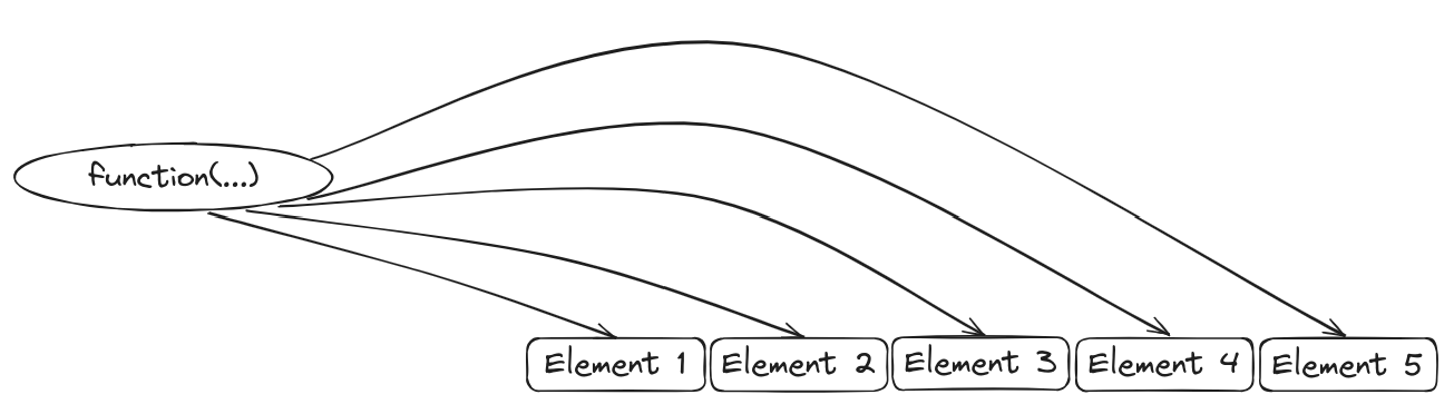
Consider an operation, that you want to apply to each element of a list. You have 3 options: Write code for each list element
Iterate over all list elements and call a function to with each element , i.e. in each iteration
Apply the function to each element directly
Easy example:
[[1]]
[1] 15

[[2]]
[1] 5050

[[3]]
[1] 500500
Data frames are just lists! So we can use this fact here. We may calculate the maximum value of each column.
'data.frame':   150 obs. of  5 variables:
 $ Sepal.Length: num  5.1 4.9 4.7 4.6 5 5.4 4.6 5 4.4 4.9 ...
 $ Sepal.Width : num  3.5 3 3.2 3.1 3.6 3.9 3.4 3.4 2.9 3.1 ...
 $ Petal.Length: num  1.4 1.4 1.3 1.5 1.4 1.7 1.4 1.5 1.4 1.5 ...
 $ Petal.Width : num  0.2 0.2 0.2 0.2 0.2 0.4 0.3 0.2 0.2 0.1 ...
$ Species : Factor w/ 3 levels "setosa","versicolor",..: 1 1 1 1 1 1 1 1 1 1 ...$Sepal.Length
[1] 7.9
$Sepal.Width
[1] 4.4
$Petal.Length
[1] 6.9
$Petal.Width
[1] 2.5sapply is basically the same as lapply, but tries to simplify the result. In our last example, this makes sense: Each element is just a number.
There is a basic apply function. It is intended to apply a function on an array. We have to specify the margin. This defines, on which axis, the function should be applied.
     [,1] [,2]
[1,]    1    4
[2,]    2    5
[3,] 3 6[1] 5 7 9[1] 6 15 [,1] [,2]
[1,] 1 4
[2,] 2 5
[3,] 3 6Warning
Apply on data frames will cast a data frame into a matrix with (as.matrix/array!)
There are a lot of other apply functions. To name some of them:
mapply (apply a function to multiple vectors/lists)
tapply (apply over ragged vectors)
pbapply (adds a progress bar, package: pbapply)
mclapply (parallel version of lapply, package: parallel)
Control flows and programming