ggplot and visualizations

Raphael Rehms

ggplot2

What is ggplot2?

• ggplot2 is a powerful data visualization package in R.
• It implements the Grammar of Graphics, allowing users to build complex plots from simple components.
• Part of the tidyverse.
• Install ggplot2

install.packages("ggplot2")

• load library in your script

library(ggplot2)

General syntax

ggplot(data = ..., mapping = aes(...)) + 
  geom_... +
  ... +
  ...

• data: the function expects a data frame
• mapping(...) Aesthetic mappings: Defines the variables that are mapped to certain visual properties with a function aes(...)
• geom_...: Geometric objects defining the type of plot

A first example: Scatterplot

• We use iris data set as an working example

library(ggplot2)
data("iris", package = "datasets")
head(iris)

  Sepal.Length Sepal.Width Petal.Length Petal.Width Species
1          5.1         3.5          1.4         0.2  setosa
2          4.9         3.0          1.4         0.2  setosa
3          4.7         3.2          1.3         0.2  setosa
4          4.6         3.1          1.5         0.2  setosa
5          5.0         3.6          1.4         0.2  setosa
6          5.4         3.9          1.7         0.4  setosa

• A scatterplot can be specified using geom_point()

ggplot(data = iris, aes(x = Sepal.Length, y = Sepal.Width))+
  geom_point()

• Note that the variable names are not in quote marks. Call them as they are actual objects.

A first example: Scatterplot

ggplot(data = iris, aes(x = Sepal.Length, y = Sepal.Width))+
  geom_point()

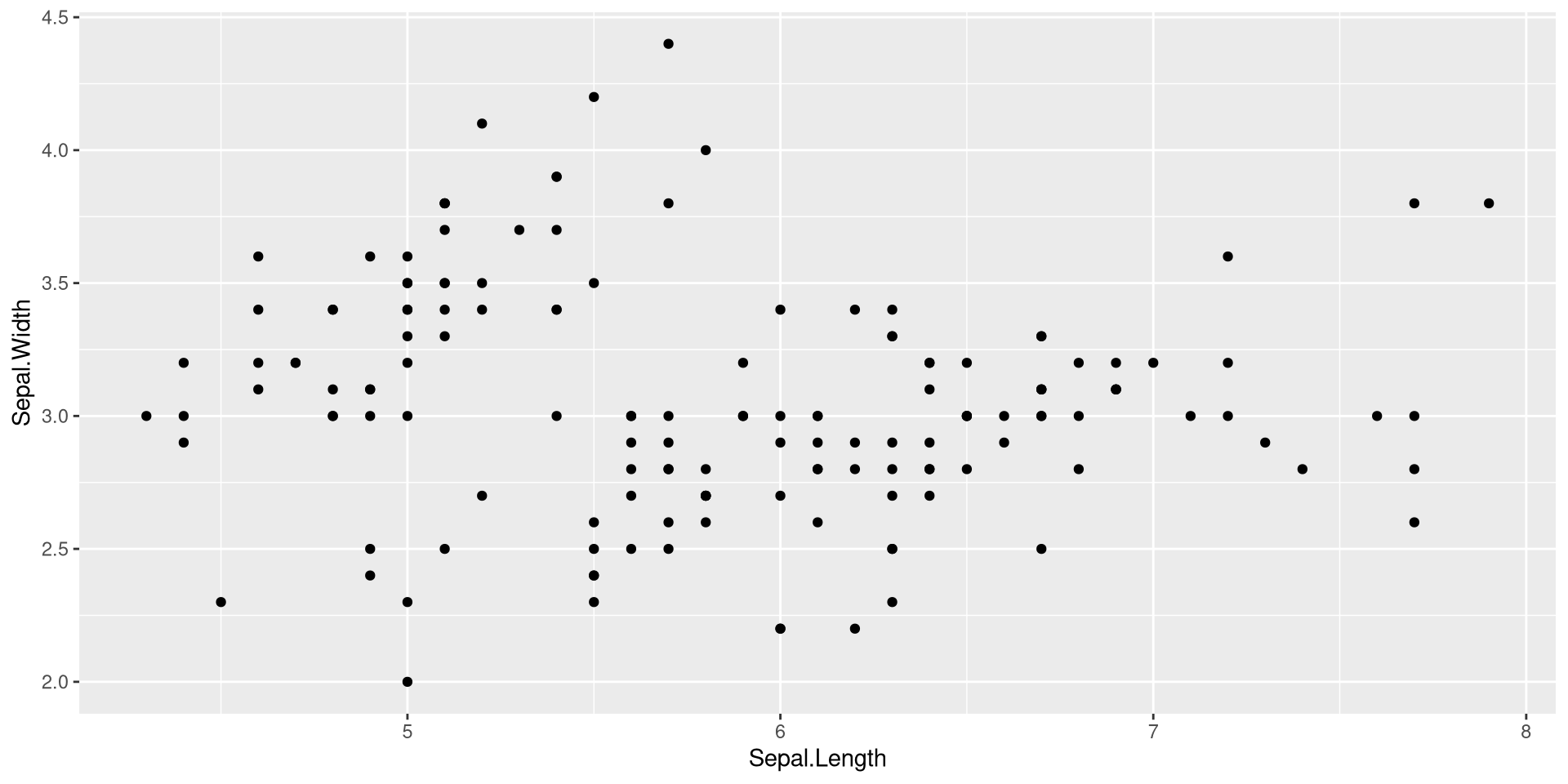
• Note that the variable names are not in quote marks. Call them as they are actual objects.

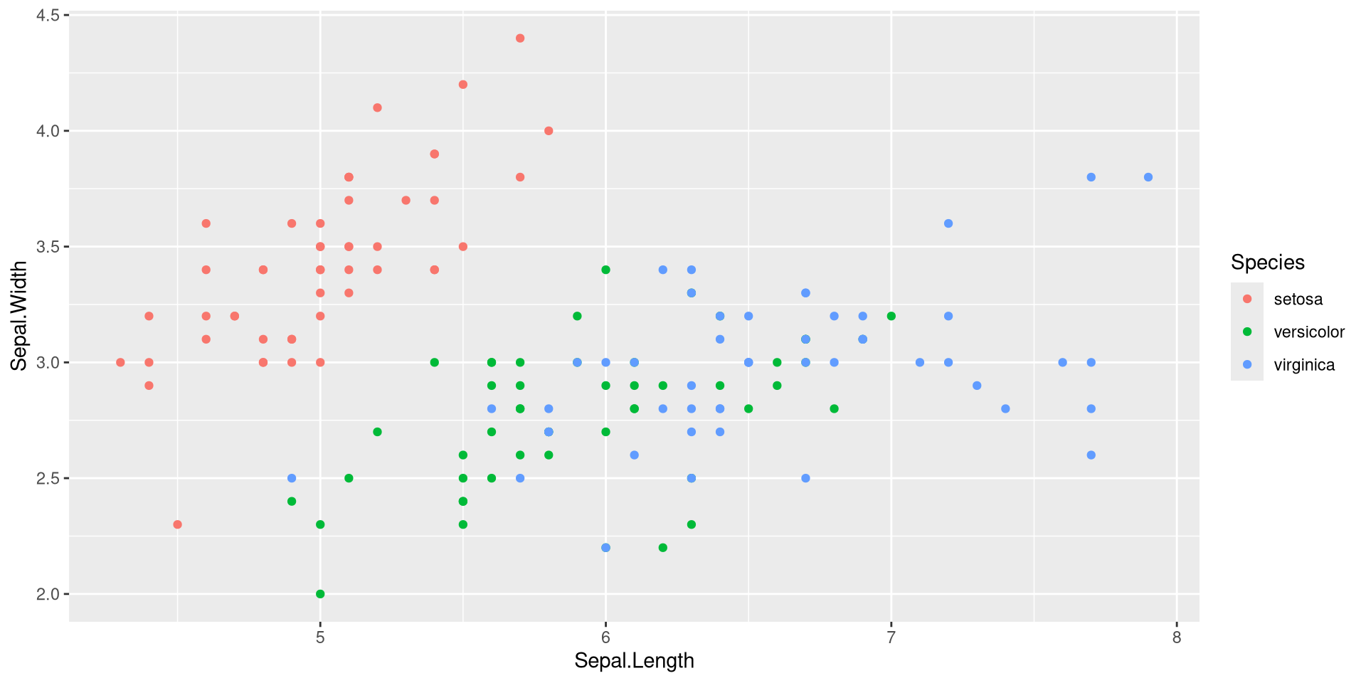
Adding another aesthetic mapping

ggplot(data = iris, aes(x = Sepal.Length, y = Sepal.Width, color = Species))+
  geom_point()

Adding color for continuous data and shape

ggplot(data = iris, aes(x = Sepal.Length, y = Sepal.Width, 
                        color = Petal.Length, shape = Species))+
  geom_point(size = 4)

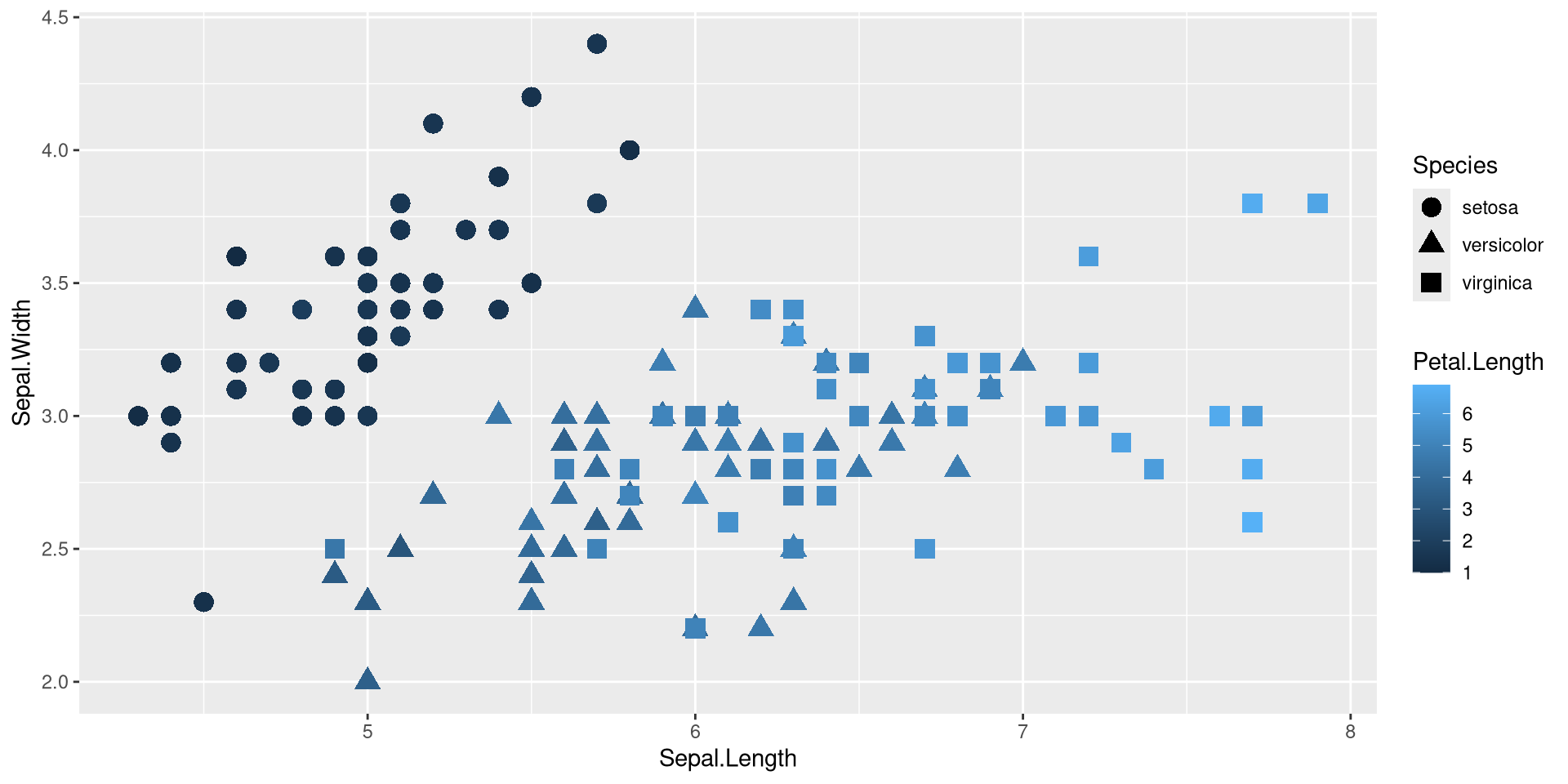
• We added a size argument to the geom_point-function to make the points larger

Exercises 3 Tasks 1

Lines

We define a simple function \[ f(x) = sin(x) + cos(x \cdot 0.5) \]

foo <- function(x) sin(x) + cos(x*0.5)
x <- seq(0, 20, len = 100)
y <- foo(x)

• We now deliberately ignore the data argument in ggplot and just define x and y.

ggplot(mapping = aes(x = x, y = y))+
  geom_line()

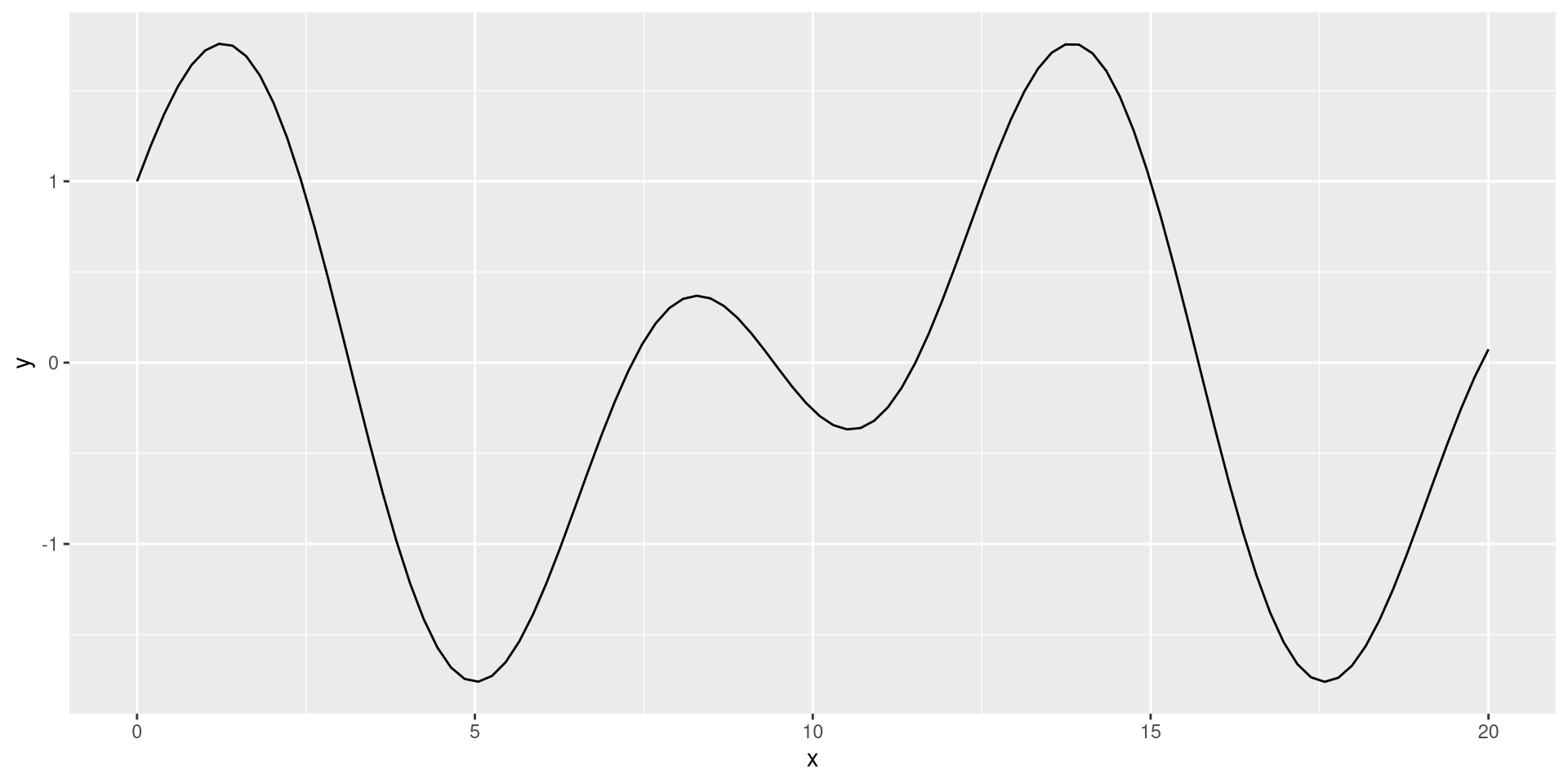
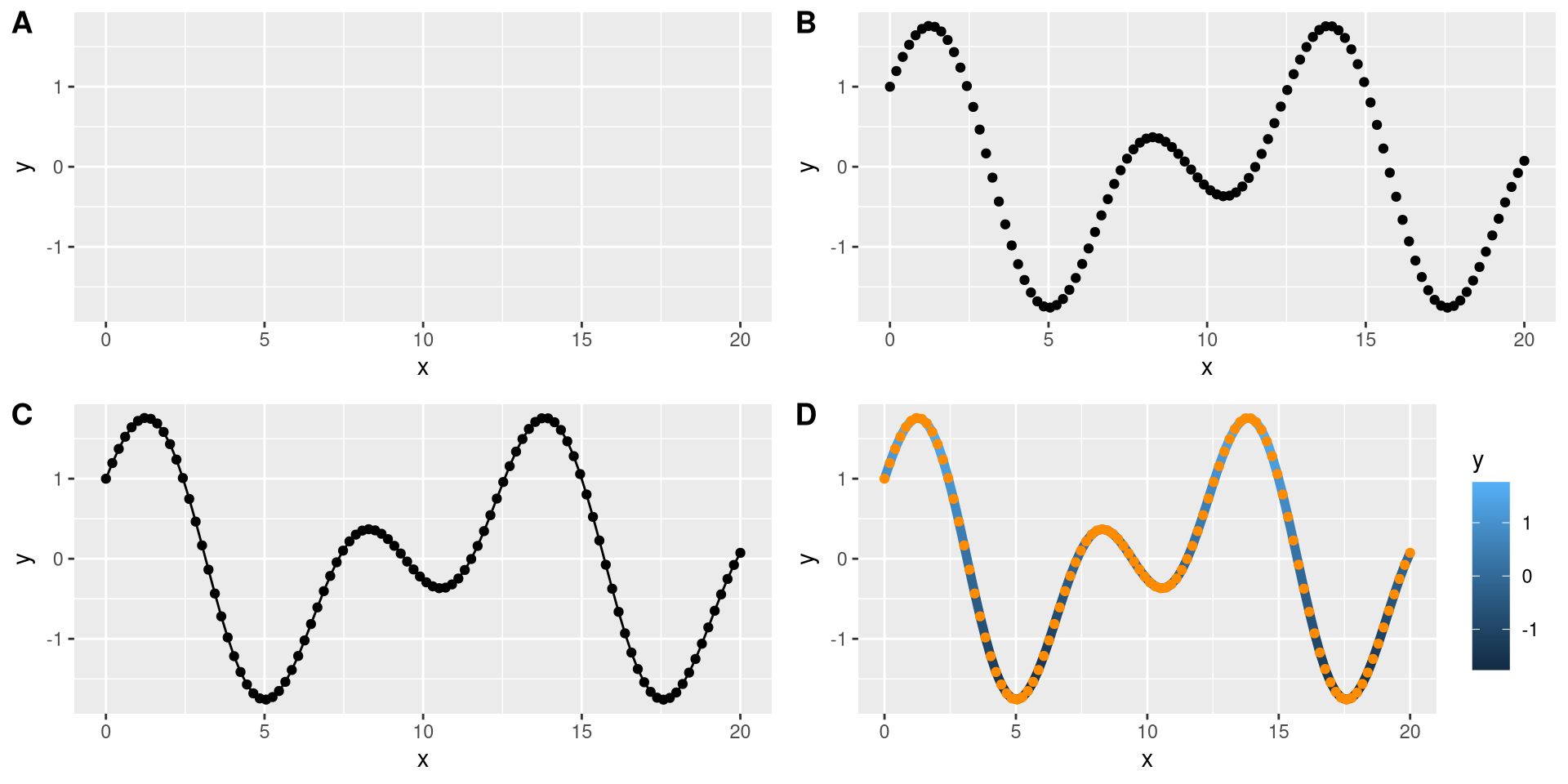
Lines

ggplot(mapping = aes(x = x, y = y))+
  geom_line()

ggplot objects

• We can assign the ggplot as an object…

g <- ggplot(mapping = aes(x = x, y = y))

• and look at it:

g

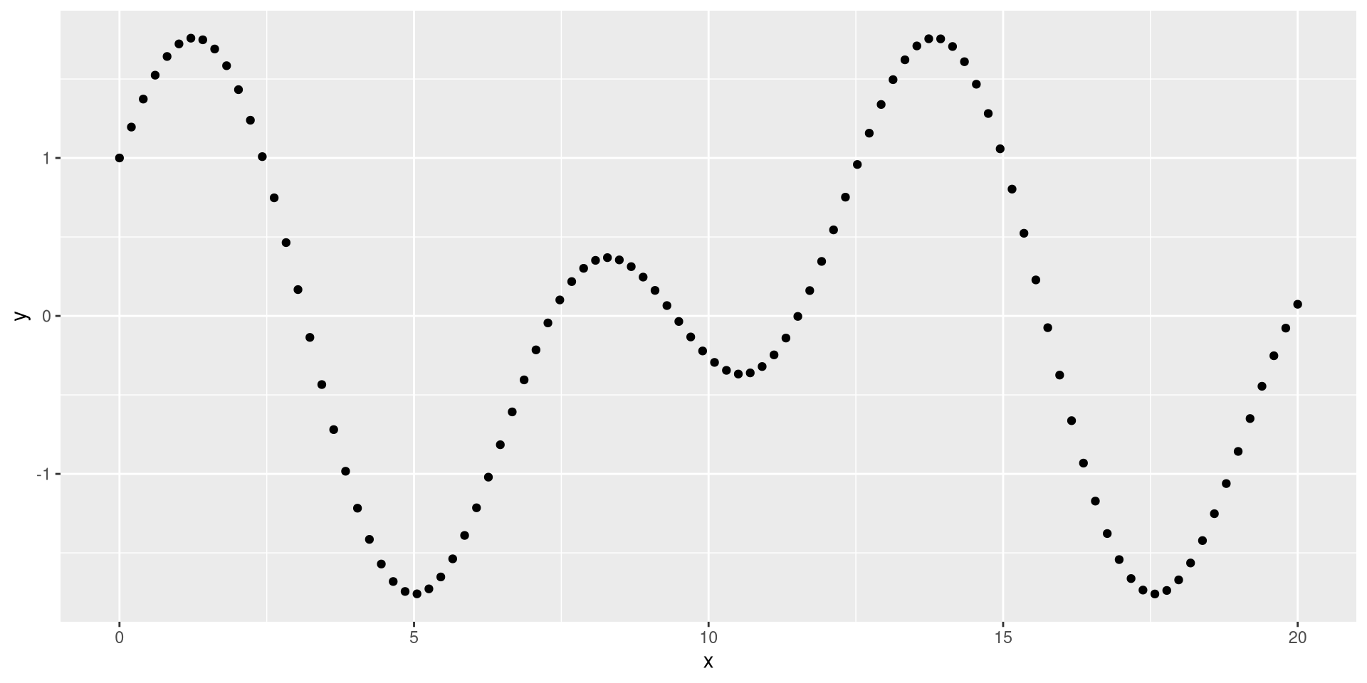
ggplot objects

• adding layers later to an object:

g +
  geom_point()

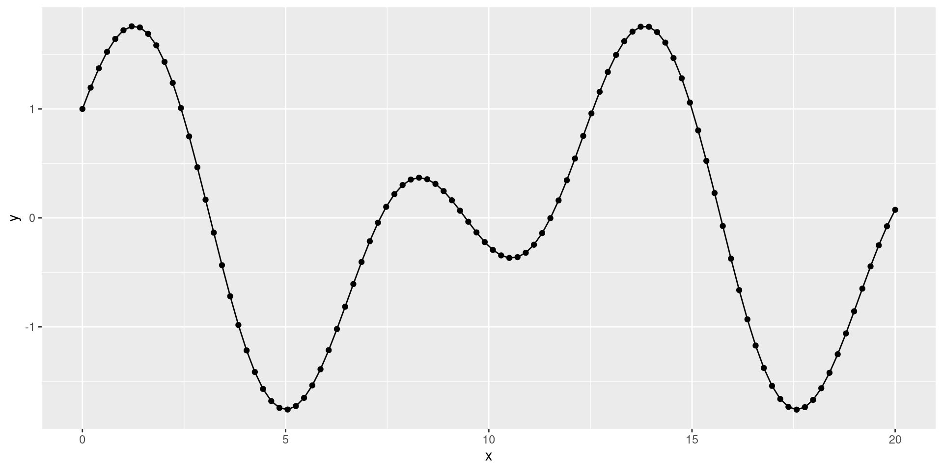
add multiple layers

g +
  geom_point()+
  geom_line()

Subplots

Multiple plots can be designed using external packages. Here, we use cowplot.

library(cowplot)

# assign two objects
g_point <- g +
  geom_point()

g_point_line <- g +
  geom_point()+
  geom_line()

g_point_line_color <- g + 
  geom_line(aes(color = y), linewidth=2)+
  geom_point(color = "darkorange")

plot_grid(g, g_point, g_point_line, g_point_line_color,
          nrow = 2, ncol = 2,
          labels="AUTO")

Note that we have different color arguments:

• In line 12 inside aes(...) with a variable name

• In line 13 outside of aes(...)

• Control line width accordingly using linewidth (here: outside aes(...) )

Subplots

Exercises 3 Tasks 2

Other types of plot

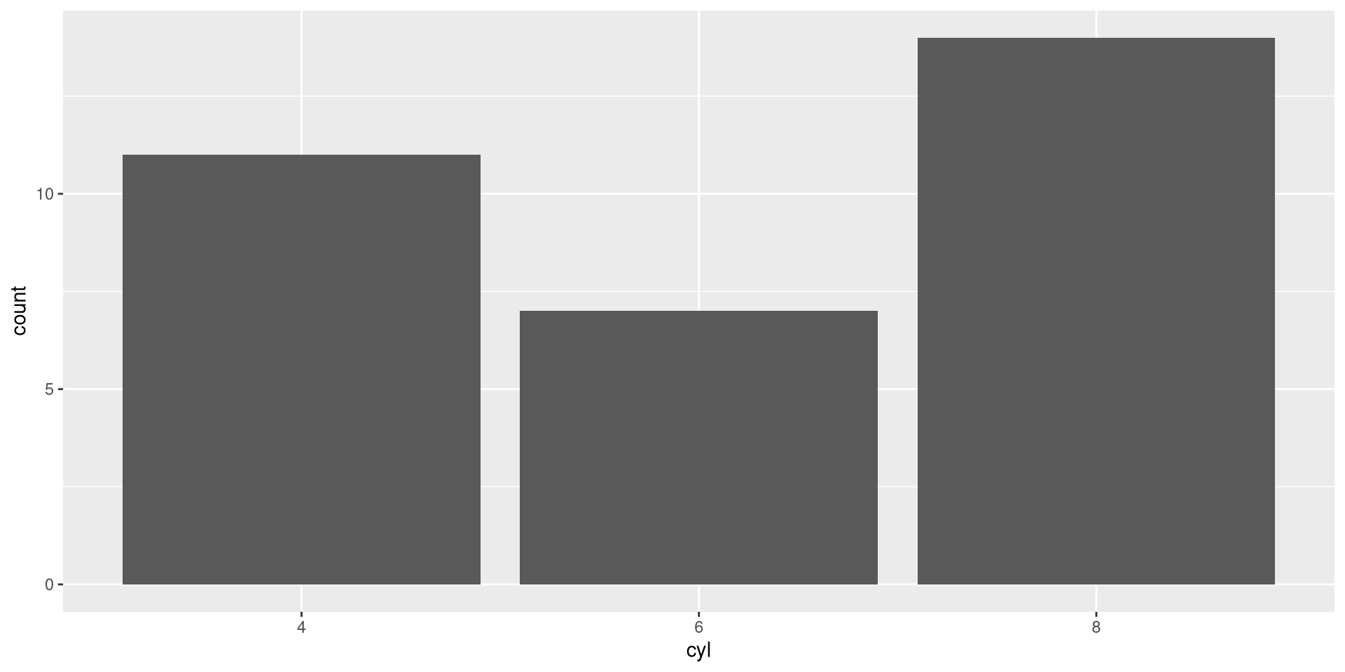
Barplot

The syntax stays the same for a type of plots. - A barplot only requires aesthetics for x. - We use the mtcars data set as an example

data <- mtcars
data$cyl <- as.factor(data$cyl)
ggplot(data, aes(cyl))+
  geom_bar()

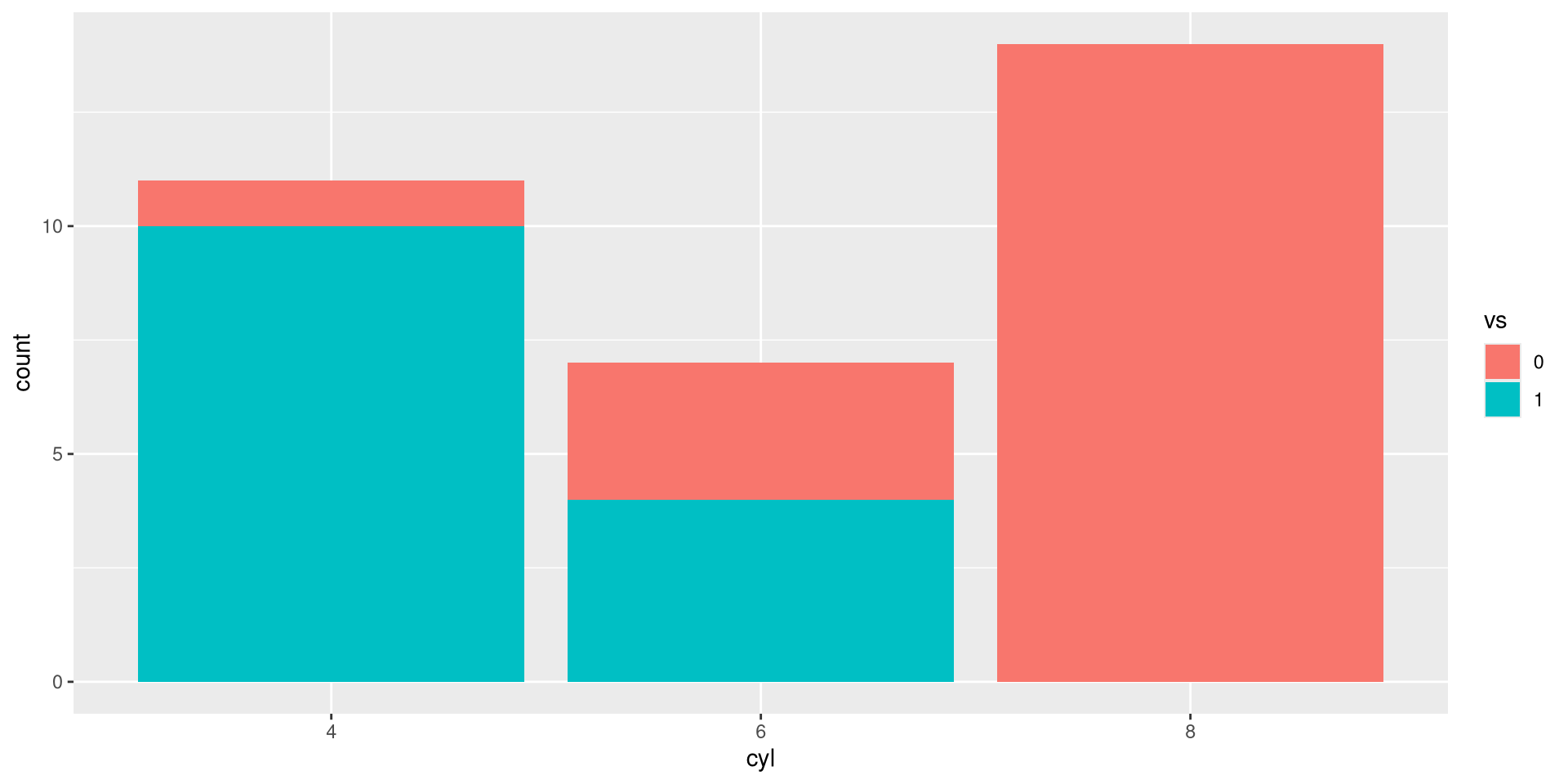
Add color

Use fill instead of color here.

data$vs <- as.factor(data$vs)
ggplot(data, aes(cyl, fill = vs))+
  geom_bar()

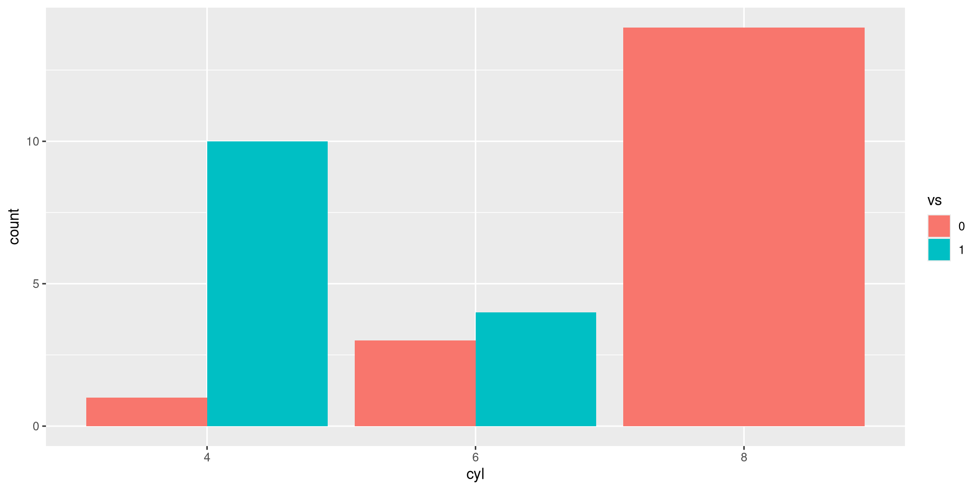
Add color

Side by side:

data$vs <- as.factor(data$vs)
ggplot(data, aes(cyl, fill = vs))+
  geom_bar(position = "dodge")

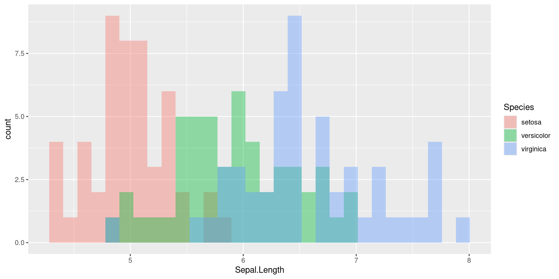
Histogram

Here, we use iris again. - position = "identity" to overplot histograms

ggplot(iris, aes(Sepal.Length, fill = Species))+
  geom_histogram(bins = 30, alpha = 0.4, position = "identity") # alpha for transparency

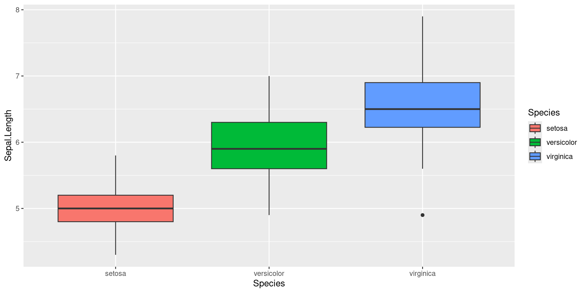
Boxplot

• Note that we have Species on the x-axis and as fill color

ggplot(iris, aes(x = Species, y = Sepal.Length, fill = Species))+
  geom_boxplot()

Violin

ggplot(iris, aes(x = Species, y = Sepal.Length, fill = Species))+
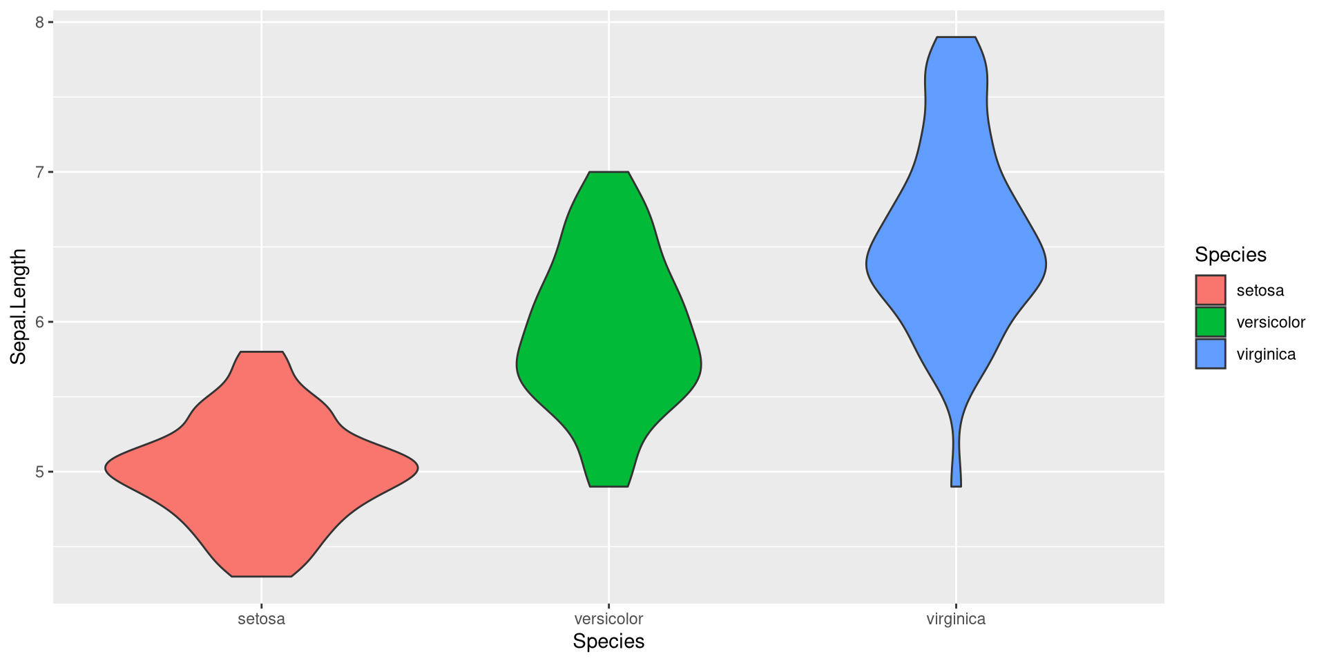
  geom_violin()

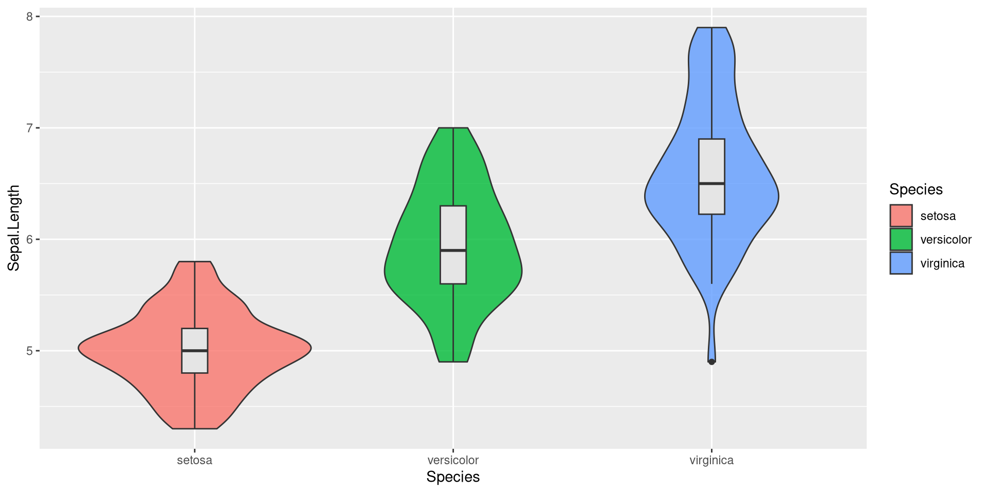
Combination

ggplot(iris, aes(x = Species, y = Sepal.Length, fill = Species))+
  geom_violin(alpha = 0.8)+
  geom_boxplot(width=0.1, fill="grey90")

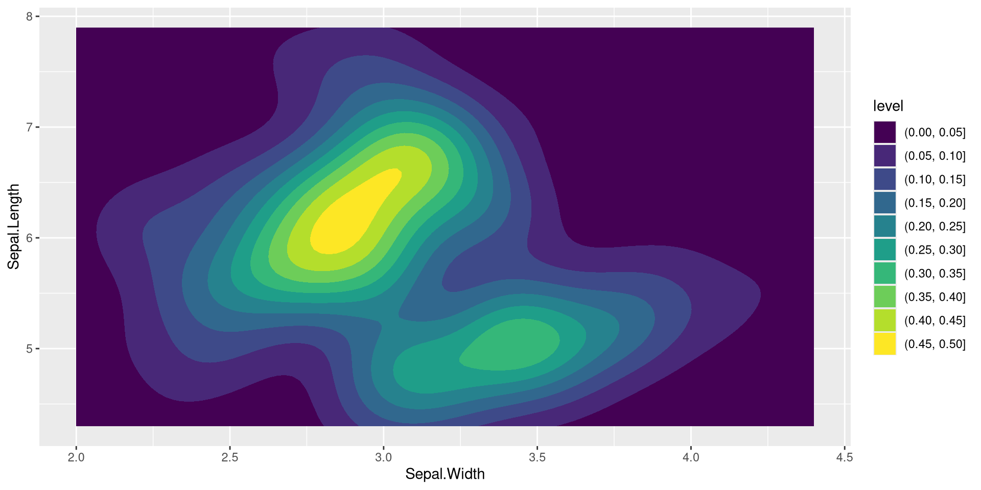
2-dim density

ggplot(iris, aes(x = Sepal.Width, y = Sepal.Length))+
  geom_density2d_filled()

Exercises 3 Tasks 3