gtsummary

Creating Summary Tables

Introduction

• An R package designed to create professional, publication-ready summary tables.

• Generates summary tables, including descriptive statistics, regression results, and statistical tests.

• Primarily used in medical and statistical reporting but versatile for a variety of applications.

Note

relies on other packages such as dplyr, purr, tidyverse so install these prior

Key features

• Generates summary statistics like mean, median, standard deviation, etc automatically.

• Supports linear, logistic, and Cox proportional hazards regression

• Allows users to modify table appearance and content as per their needs.

install and load package

library(gtsummary)
library(gt)
library(mgcv)
library(broom)
library(dplyr)
library(tidyr)

we use air quality data set as an working example

data("mtcars", package = "datasets")
 mydata <- mtcars
head(mydata)

                   mpg cyl disp  hp drat    wt  qsec vs am gear carb
Mazda RX4         21.0   6  160 110 3.90 2.620 16.46  0  1    4    4
Mazda RX4 Wag     21.0   6  160 110 3.90 2.875 17.02  0  1    4    4
Datsun 710        22.8   4  108  93 3.85 2.320 18.61  1  1    4    1
Hornet 4 Drive    21.4   6  258 110 3.08 3.215 19.44  1  0    3    1
Hornet Sportabout 18.7   8  360 175 3.15 3.440 17.02  0  0    3    2
Valiant           18.1   6  225 105 2.76 3.460 20.22  1  0    3    1

Make sure that the class of each variable are correct.

str(mydata)
#I want cyl, vs, am, gear to be factor, and all other numeric
mydata$cyl <- as.factor(mydata$cyl)
mydata$vs <- as.factor(mydata$vs)
mydata$gear <- as.factor(mydata$gear)
mydata$carb <- as.factor(mydata$carb)
mydata$am <- as.factor(mydata$am)

First Example: Descriptive table

simple <- mydata %>%
  select(mpg,hp, qsec, vs, gear) %>%
  tbl_summary()

simple

select() only selects the specified columns, is a part of dplyr package

tbl_summary() generates a summary table that shows descriptive statistics for each variable.

First Example: Descriptive table

Characteristic	N = 321
mpg	19.2 (15.4, 22.8)
hp	123 (96, 180)
qsec	17.71 (16.89, 18.90)
vs
0	18 (56%)
1	14 (44%)
gear
3	15 (47%)
4	12 (38%)
5	5 (16%)
1 Median (Q1, Q3); n (%)

Formatting and styling

descriptive <- mydata %>%
  select(mpg,hp, qsec, vs, gear) %>%
  tbl_summary( by = "vs") %>%
  modify_header(label ~ "Variable")


descriptive

by = “vs” groups the data by the variable vs

By default, the summary table labels the first column (the variable names) as label.

We use modify_header to rename this column to “Variable” so that it looks more professional and understandable.

Formatting and styling

Variable	0 N = 181	1 N = 141
mpg	15.7 (14.7, 19.2)	22.8 (21.4, 30.4)
hp	180 (150, 230)	96 (66, 110)
qsec	17.02 (15.84, 17.42)	19.17 (18.60, 20.00)
gear
3	12 (67%)	3 (21%)
4	2 (11%)	10 (71%)
5	4 (22%)	1 (7.1%)
1 Median (Q1, Q3); n (%)

More features

add mean and standard deviation instead of quartiles, change column/row percentage

descriptive <- mydata %>%
  select(mpg,hp, qsec, vs, gear) %>%
  tbl_summary(
  by = "vs", 
  statistic = list(
    all_continuous() ~ "{mean} ({sd})",
    all_dichotomous() ~ "{n} ({p}%)",
    all_categorical() ~ "{n} ({p}%)"
  ),
  missing = "no",
  percent = "column",  # You can change this to "row" if you want row percentages instead
  digits = list(all_categorical() ~ c(0, 1))
) %>%
  modify_header(label ~ "Variable")

descriptive

• statistic=, defines the type of statistic we want to calculate for each type of variable.
• By default missing values are counted and we can use missing = “no” argument to exclude missing value from the summmary.
• percent= “column” calculates percentages within each column. You can change this to “row” if you want percentages calculated within each row.
• The number inside ~ c(0,1), defines the number of decimal place for two different elements. First (0) sets the decimal place for counts and second (1) for percentages.

More features

Variable	0 N = 181	1 N = 141
mpg	16.6 (3.9)	24.6 (5.4)
hp	190 (60)	91 (24)
qsec	16.69 (1.09)	19.33 (1.35)
gear
3	12 (66.7%)	3 (21.4%)
4	2 (11.1%)	10 (71.4%)
5	4 (22.2%)	1 (7.1%)
1 Mean (SD); n (%)

Adding Statistical Tests

descriptive <- mydata %>%
  select(mpg,hp, qsec, vs, gear) %>%
  tbl_summary( 
    by = "vs",
    statistic = list(
      all_continuous() ~ "{mean} ({sd})",
      all_dichotomous() ~ "{n} ({p}%)",
      all_categorical() ~ "{n} ({p}%)"
    ),
    missing = "no",
    percent = "column",
    digits = list(all_categorical() ~ c(0, 1))
  ) %>%
  add_overall() %>% # Add overall column
  add_p(
    test = list(
      all_continuous() ~ "t.test", # t-test for continuous variables
      all_categorical() ~ "chisq.test" # chi-square test for categorical variables
    ),
    pvalue_fun = ~style_pvalue(.x, digits = 3) # Optionally set the number of digits for p-values
  ) %>%
  modify_header(label ~ "**Variable**") %>% # Modify the header
  modify_spanning_header(c("stat_0", "stat_1", "stat_2") ~ "**VS**") %>%
  bold_labels()
  
descriptive

• add_overall(), adds an extra column to the table that shows statistics for the entire dataset
• add_p(), argument performs statistical test for checking whether the differences between the vs groups are statistically significant
• pvalue_fun formats the p-values to 3 decimal places
• modify_spanning_header(c(“stat_0”, “stat_1”, “stat_2”) ~ “VS”), creates a single, bolded header labeled VS that spans across the specified columns

Adding Statistical Tests

Variable	VS			p-value
	Overall N = 321	0 N = 181	1 N = 141
mpg	20.1 (6.0)	16.6 (3.9)	24.6 (5.4)
hp	147 (69)	190 (60)	91 (24)
qsec	17.85 (1.79)	16.69 (1.09)	19.33 (1.35)
gear
3	15 (46.9%)	12 (66.7%)	3 (21.4%)
4	12 (37.5%)	2 (11.1%)	10 (71.4%)
5	5 (15.6%)	4 (22.2%)	1 (7.1%)
1 Mean (SD); n (%)

Making table more publication ready

descriptive_modified <- descriptive %>%
  as_gt() %>%
  gt::tab_options(
    table.font.size = "small",
    heading.title.font.size = "medium",
    heading.subtitle.font.size = "small"
  ) %>%
  gt::tab_header(
    title = "Descriptive Analysis of mtcars"
  ) %>%
  gt::cols_align(
    align = "center",
    columns = everything()
  ) %>%
  gt::tab_style(
    style = cell_borders(
      sides = "bottom",
      color = "black",
      weight = px(2)
    ),
    locations = cells_body(
      columns = everything(), # style to all columns in the table, not just specific ones
      rows = c(1, 2, 3,7)  # bottom border will only be applied to
    )
  ) %>%
  gt::tab_style(
    style = cell_text(weight = "bold"), # Makes the text of row group labels bold.
    locations = cells_row_groups()
  )

descriptive_modified

• as_gt(), is a part of gt package focused on table formatting.This changes descriptive table from gtsummary package into a gt object
• gt::tab_header(), for adding the title to the table
• gt::cols_align(), centers all the columns in the table for uniformity
• gt::tab_style(…), to customize styles according to your preference. We can apply variety of styles to different part of table other than shown in the example. Such as changing the font style, size, text colour, backround colour, conditional formatting and all.

Making table more publication ready

Descriptive Analysis of mtcars
Variable	VS			p-value
	Overall N = 321	0 N = 181	1 N = 141
mpg	20.1 (6.0)	16.6 (3.9)	24.6 (5.4)
hp	147 (69)	190 (60)	91 (24)
qsec	17.85 (1.79)	16.69 (1.09)	19.33 (1.35)
gear
3	15 (46.9%)	12 (66.7%)	3 (21.4%)
4	12 (37.5%)	2 (11.1%)	10 (71.4%)
5	5 (15.6%)	4 (22.2%)	1 (7.1%)
1 Mean (SD); n (%)

Advanced Features

Regression Tables

mod<- lm(mpg ~ vs + hp +gear, data = mydata)
tbl_regression(mod)

• table regression, automatically takes the output of a regression model and presents a summary of the model’s results in a table format.

Now you can format the tables as you like by adding more commands

Regression Tables

Characteristic	Beta	95% CI1	p-value
vs
0	—	—
1	1.8	-1.7, 5.2	0.3
hp	-0.06	-0.09, -0.03	<0.001
gear
3	—	—
4	2.2	-1.2, 5.5	0.2
5	6.4	3.1, 9.8	<0.001
1 CI = Confidence Interval

Formatting

table_model <- tbl_regression(
  mod
) %>%
  add_global_p(anova_fun = gtsummary::tidy_wald_test) 
table_model

• adds a global p-value to the regression summary table
• gtsummary::tidy_wald_test: This function from the gtsummary package calculates the Wald test for the overall model, we can use likelyhood ratio test, f-test, score test.

Formatting

Characteristic	Beta	95% CI1	p-value
vs			0.3
0	—	—
1	1.8	-1.7, 5.2
hp	-0.06	-0.09, -0.03	<0.001
gear			<0.001
3	—	—
4	2.2	-1.2, 5.5
5	6.4	3.1, 9.8
1 CI = Confidence Interval

Tip

For logistic models you can add exponentiate = TRUE, command to get the odds ratio

Merging Tables

mod1<- lm(qsec ~ vs + hp +gear, data = mydata)

table_model_1 <- tbl_regression(
  mod1
) %>%
  add_global_p(anova_fun = gtsummary::tidy_wald_test) 

# Merge the regression tables for comparison
comparison_table <- tbl_merge(
  tbls = list(table_model, table_model_1),
  tab_spanner = c("Model1","Model2")
)

comparison_table

tbl_merge(), combines multiple summary table into one tab_spanner allows to label the columns that comes from the two table

Merging Tables

Characteristic	Model1			Model2
	Beta	95% CI1	p-value	Beta	95% CI1	p-value
vs			0.3			<0.001
0	—	—		—	—
1	1.8	-1.7, 5.2		2.0	0.92, 3.0
hp	-0.06	-0.09, -0.03	<0.001	-0.01	-0.02, 0.00	0.047
gear			<0.001			<0.001
3	—	—		—	—
4	2.2	-1.2, 5.5		-0.66	-1.7, 0.34
5	6.4	3.1, 9.8		-1.9	-2.9, -0.88
1 CI = Confidence Interval

comparison_table_final <- as_gt(comparison_table) %>%
  gt::tab_options(
    table.font.size = "small",
    heading.title.font.size = "medium",
    heading.subtitle.font.size = "small"
  ) %>%
  gt::tab_header(
    title = "Model Comparison"
  ) %>%
  gt::cols_align(
    align = "center",
    columns = everything()
  ) %>%
  gt::tab_style(
    style = cell_text(weight = "bold"),
    locations = cells_column_labels(
      columns = everything()
    )
  ) %>%
  gt::tab_style(
    style = cell_borders(
      sides = "bottom",
      color = "black",
      weight = px(2)
    ),
    locations = cells_body(
      columns = everything(),
      rows = c(3, 4, 5,8)  
    )
  ) %>%
  gt::tab_style(
    style = cell_text(weight = "bold"),
    locations = cells_row_groups()
  )

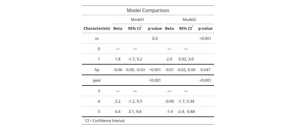
comparison_table_final

Model Comparison
Characteristic	Model1			Model2
	Beta	95% CI1	p-value	Beta	95% CI1	p-value
vs			0.3			<0.001
0	—	—		—	—
1	1.8	-1.7, 5.2		2.0	0.92, 3.0
hp	-0.06	-0.09, -0.03	<0.001	-0.01	-0.02, 0.00	0.047
gear			<0.001			<0.001
3	—	—		—	—
4	2.2	-1.2, 5.5		-0.66	-1.7, 0.34
5	6.4	3.1, 9.8		-1.9	-2.9, -0.88
1 CI = Confidence Interval

Saving tables

#saving into word document 
gtsave(comparison_table_final, "table.docx")


# Save the gt table as an HTML file
gtsave(comparison_table_final, "table.html")

# Capture the HTML file as an image using webshot2
webshot2::webshot("table.html", file = "table.png", vwidth = 1000, vheight = 800)

• gtsave() saves a gtsummary or gt table to a file in various formats
• webshot2::webshot() takes a screenshot of an HTML file or webpage and saves it as an image