[1] 3[1] -1[1] 2[1] 0.5[1] 1Why R?
R is open source
All techniques for data analyses
State-of-the-art graphics capabilities
A platform for programming new statistical methods or analysis pipelines (in form of R-packages)
“Good programmers are made, not born.” (Gerald M. Weinberg - The Psychology of Computer Programming)
consequence I
train…
consequence II
train…
consequence III
train more
Hands-on is important. Understanding is less that 30%
Required tools for the course:
Programming language R
RStudio (optional, but recommended)
IDE tailored for R
Integrates a lot more (e.g. python, c++, etc.)
R comes with many useful packages by default
However, the strength lies in the huge collection of external packages
Most popular and default: CRAN
Install new packages in R using either
using a command:
install.packages("<package-name>") (e.g.install.packages("mvtnorm"))RStudio
Special symbols
Mathematical functions
Special cases:
NaN is a data type that indicates an invalid number.NA is a missing value.NULL means literally empty/nothingAssignment is done using <-
Alternatively, use =
Look at environment pane in R Studio, what can you see?
R have to start with a letterCase sensitive
Overwrite variables with old ones
Combination of words
So far we used expressions like f(...). This is a function. E.g.
We call the function exp with a value of 2. Or the (natural) logarithm:
We can specify the base as a second argument:
Access the documentation using
<F1>
type ?function_name
use RStudio functionality
E.g. documentation for log() reveals that we calculate the natural logarithm.
You can ignore the argument name, when placements are clear. - We have done that for exp and log
Hence, this here
means, that we actually call
If you specify the argument, order does not matter.
Example:
numericA (floating point) number. We used this so far (default).
1.0, 1.34, -33, pi
logicalA binary data type.
TRUE, FALSE, T, F
integerCan be specified using an “L”.
1L, 100L, -99L
characterRepresents letters OR sentences.
'a', "abc", "May the force be with you"
You can combine single values to a vector.
[1] 1 2 3 4[1] TRUE FALSE TRUE[1] "a" "ab" "ab c"Many operations in R are vectorized
[1] 2 4 6 8[1] 1 4 9 16[1] 2.718282 7.389056 20.085537 54.598150[1] -1 -2 -3 -4NA or NaNs can be part of a vectorThere are a lot of convenience functions to create vectors.
More complex ones:
Access elements of a vector using positional numbers within [...]:
Multiple elements
Negative values will be excluded
Recall the very most basic data type logical, i.e. TRUE and FALSE.
[1] FALSE[1] TRUE[1] FALSE[1] FALSE[1] TRUE[1] TRUESwap value:
Comparison operators are vectorized:
Check condition on a numeric vector
x <- c(2,4,2,5)
position_two <- x == 2  # logical vector showing, where the condition holds
position_two
[1] TRUE FALSE TRUE FALSEUse logical values to filter a vector.
Filter for values less than 3
& and |Combination operations…
…or vectorized
Use this to filter a vector for multiple conditions
We can assign new values to a vector using a combination of selection and assignment
[1] 2 2 3 4 5[1] 2 2 3 -99 -99[1] 2 100 100 100 100Consider a vector, that represents a categorical variable. Let’s say colors.
[1] "blue" "red" "blue" "red" "green" "black" "green" "white"We cast colors into a factor now:
[1] blue  red   blue  red   green black green white
Levels: black blue green red white[1] "black" "blue" "green" "red" "white"[1] 2 4 2 4 3 1 3 5[1] "factor"[1] "integer"Hence, a vector of integeres where each value corresponds to a character value.
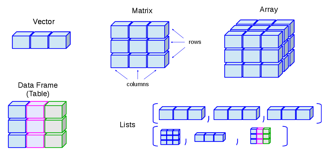
from *Ceballos and Cardiel, (2013). Data structure – First Steps in R. Retreived 25-11-2018 from http://venus.ifca.unican.es/Rintro/_images/dataStructuresNew.png*
Use str(...) to inspect the structure of complex data types!
We already got vectors. Lets combine them:
We can define a matrix using the matrix function:
     [,1] [,2]
[1,]    1    4
[2,]    2    5
[3,] 3 6 [,1] [,2]
[1,] 1 2
[2,] 3 4
[3,] 5 6Arrays as a generalization with multiple dimensions
, , 1

     [,1] [,2]
[1,]    1    4
[2,]    2    5
[3,]    3    6

, , 2

     [,1] [,2]
[1,]    7   10
[2,]    8   11
[3,]    9   12
This is also sometimes called a tensor.
As vectors, we can select and filter. Seperate dimensions with a ,, i.e. [... , ...]
     [,1] [,2]
[1,]    1    4
[2,]    2    5
[3,] 3 6[1] 5[1] 6Defining no entry will return the full dimension:
A list is a collection of elements. These elements could be any object.
[[1]]
[1] 1

[[2]]
[1] "2"

[[3]]
[1] 1 2 3

[[4]]
[[4]][[1]]
     [,1] [,2]
[1,]    1    4
[2,]    2    5
[3,]    3    6
Access elements of a list with [[...]].
A sub-list can be accessed with [...].
You can define names for lists:
Access list elements using the name and a $:
[[1]]
[1] 1

[[2]]
[1] "2"

[[3]]
[1] 1 2 3
[[4]]
[[4]][[1]]
[,1] [,2]
[1,] 1 4
[2,] 2 5
[3,] 3 6Delete elements by assigning a NULL to a slot
A data frame is basically a list, where each element is a vector of the same length. However, it implements function to handle it as a matrix.
Let’s define a data set representing cars:
col <- as.factor(c("blue", "red", "blue", "red", "green", "black", "green", "white"))
pri <- c(10, 20, 9, 50, 0.4, 15, 160, 60) * 1000
is_el <- c(F,F,F,T,F,T,F,T)

car_ds <- data.frame(color = col, price = pri, is_electric = is_el)
car_ds
color price is_electric
1 blue 10000 FALSE
2 red 20000 FALSE
3 blue 9000 FALSE
4 red 50000 TRUE
5 green 400 FALSE
6 black 15000 TRUE
7 green 160000 FALSE
8 white 60000 TRUE'data.frame': 8 obs. of 3 variables:
$ color : Factor w/ 5 levels "black","blue",..: 2 4 2 4 3 1 3 5
$ price : num 10000 20000 9000 50000 400 15000 160000 60000
$ is_electric: logi FALSE FALSE FALSE TRUE FALSE TRUE ...We can work on a data set as we work with a matrix
  color price is_electric
2   red 20000       FALSE
4 red 50000 TRUE[1] 15000 color price is_electric
1 blue 10000 FALSE
2 red 20000 FALSE
3 blue 9000 FALSE
4 red 50000 TRUE
5 green 400 FALSE
6 black 15000 TRUE
7 green 160000 FALSE
8 white 600 TRUEUse str(...) to check the data structure of any object:
We can load a data set from a package using data(...).
We can load data from files. Use read.table(...), or wrapper functions with reasonable default values. E.g. We can read a file directly from the web:
d <- read.csv("https://raw.githubusercontent.com/vincentarelbundock/Rdatasets/master/csv/datasets/mtcars.csv")
head(d)  # show the first few lines of a data set
rownames mpg cyl disp hp drat wt qsec vs am gear carb
1 Mazda RX4 21.0 6 160 110 3.90 2.620 16.46 0 1 4 4
2 Mazda RX4 Wag 21.0 6 160 110 3.90 2.875 17.02 0 1 4 4
3 Datsun 710 22.8 4 108 93 3.85 2.320 18.61 1 1 4 1
4 Hornet 4 Drive 21.4 6 258 110 3.08 3.215 19.44 1 0 3 1
5 Hornet Sportabout 18.7 8 360 175 3.15 3.440 17.02 0 0 3 2
6 Valiant 18.1 6 225 105 2.76 3.460 20.22 1 0 3 1Note, that we can also use this to read a data set from a local directory! To do that we have to specify either the full path or define the path from the working directory. Use getwd(...) and setwd(...) to get or set the current working directory. See next slide for an example.
Consider a data set, you have worked with. You can save it using write functions.
We can again read the data as a new object:
d_loaded <- read.csv("example_data.csv")

all.equal(car_ds,d_loaded)  # test whether 2 (more complex) R object are the same
[1] "Names: 3 string mismatches"
[2] "Length mismatch: comparison on first 3 components"
[3] "Component 1: 'current' is not a factor"
[4] "Component 2: Modes: numeric, character"
[5] "Component 2: target is numeric, current is character"
[6] "Component 3: Modes: logical, numeric"
[7] "Component 3: target is logical, current is numeric" We can read other files as well. E.g. excel, SPSS, SAS, etc.
There are a lot of packages to do that.
I use the function load(...) from the rio package that tries to unify a lot of different formats.)
So far, we only worked with data frames for read and write operations. We can save general R objects using save(...) and load(...) using the .RData format.
Intro intro R
Comments
Sometimes it is useful, to comment code. Use a
#to commentStandard:
Comment a line (no output):
Comment after an expression (only
1+1gets evaluated):