Models in R

Raphael Rehms und Jonathan Christ

Linear regression

Linear model

\(Y_i =\beta_0+\beta_1 \cdot X_i+ \beta_2 \cdot X_i+...+\epsilon_i\) ,with \(\epsilon \sim N(0,\sigma^2)\)

R command: lm(formula, data, ...)

Examples of formula:

y~age+sex
y~I(log(age)) + as.factor(sex)
see ?formula for more details

Note: data must be a data.frame.

Example:

library(MASS)
data(cats)
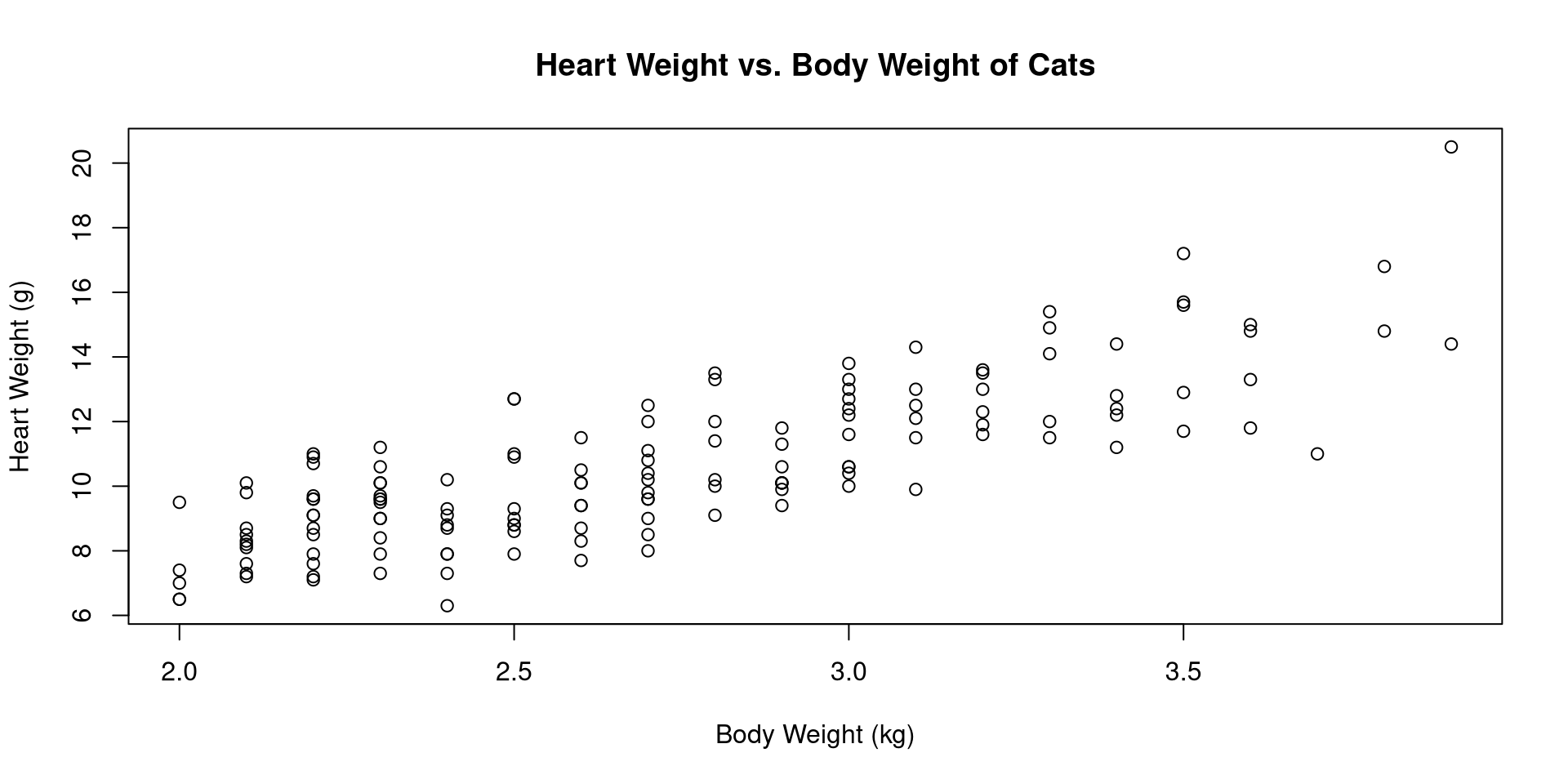
with(cats, plot(Bwt, Hwt, xlab="Body Weight (kg)",
        ylab="Heart Weight (g)",
         main="Heart Weight vs. Body Weight of Cats"))

with(cats, cor.test(Bwt, Hwt))


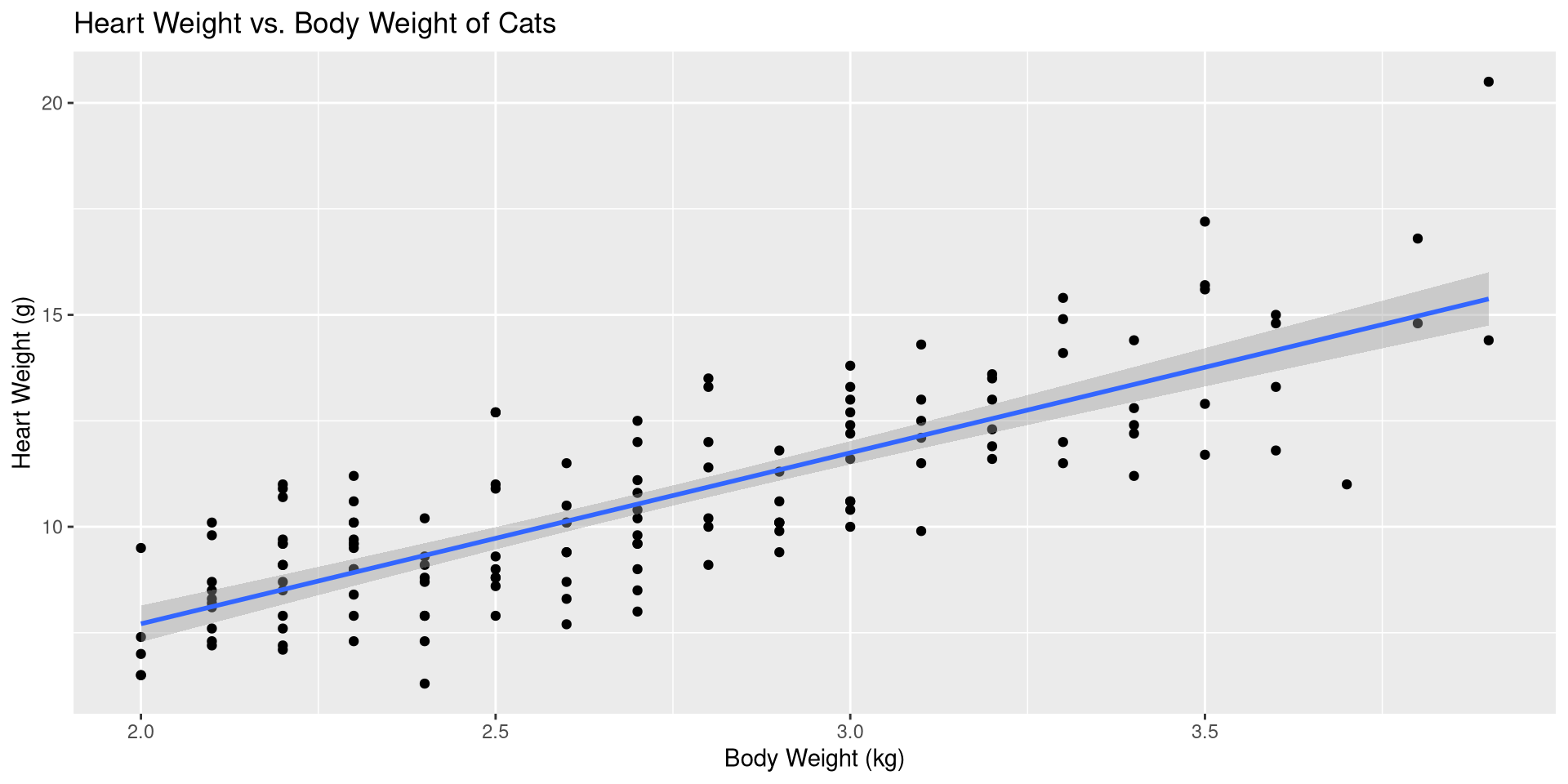
    Pearson's product-moment correlation

data:  Bwt and Hwt
t = 16.119, df = 142, p-value < 2.2e-16
alternative hypothesis: true correlation is not equal to 0
95 percent confidence interval:
 0.7375682 0.8552122
sample estimates:
      cor 
0.8041274

lm(Hwt ~ Bwt,data=cats)


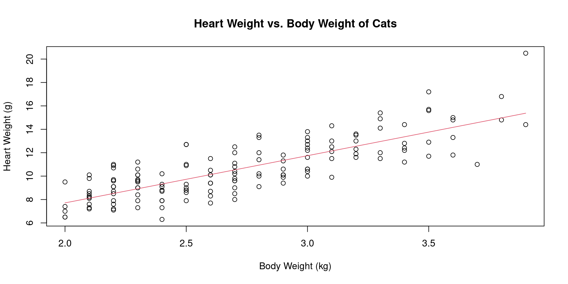
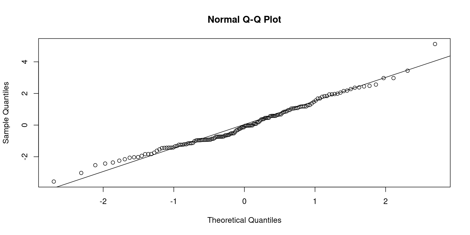
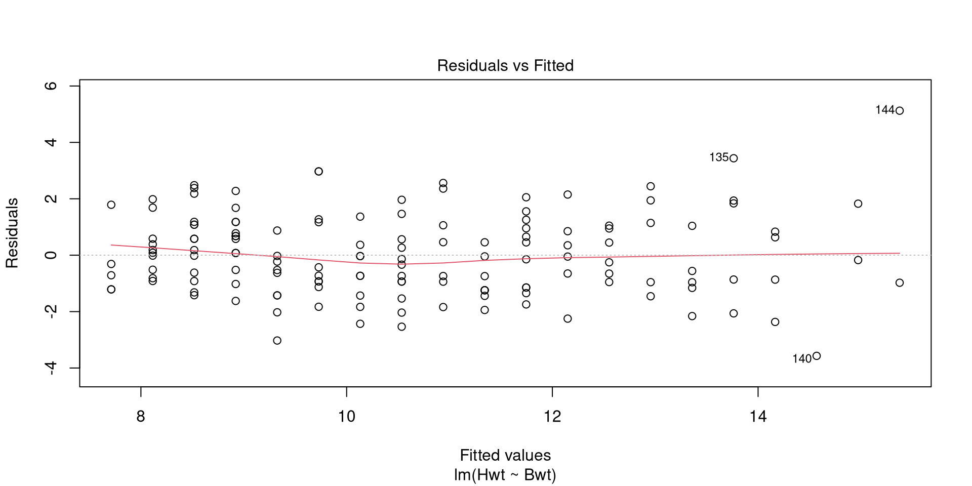
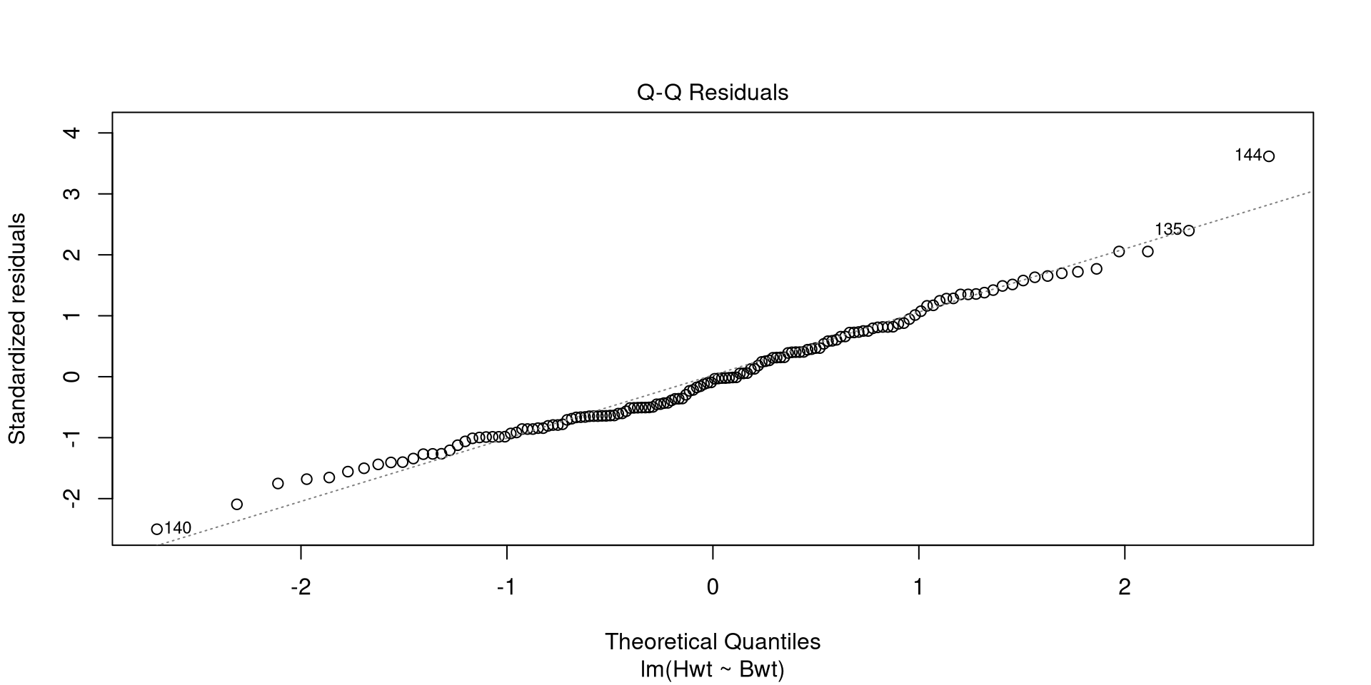
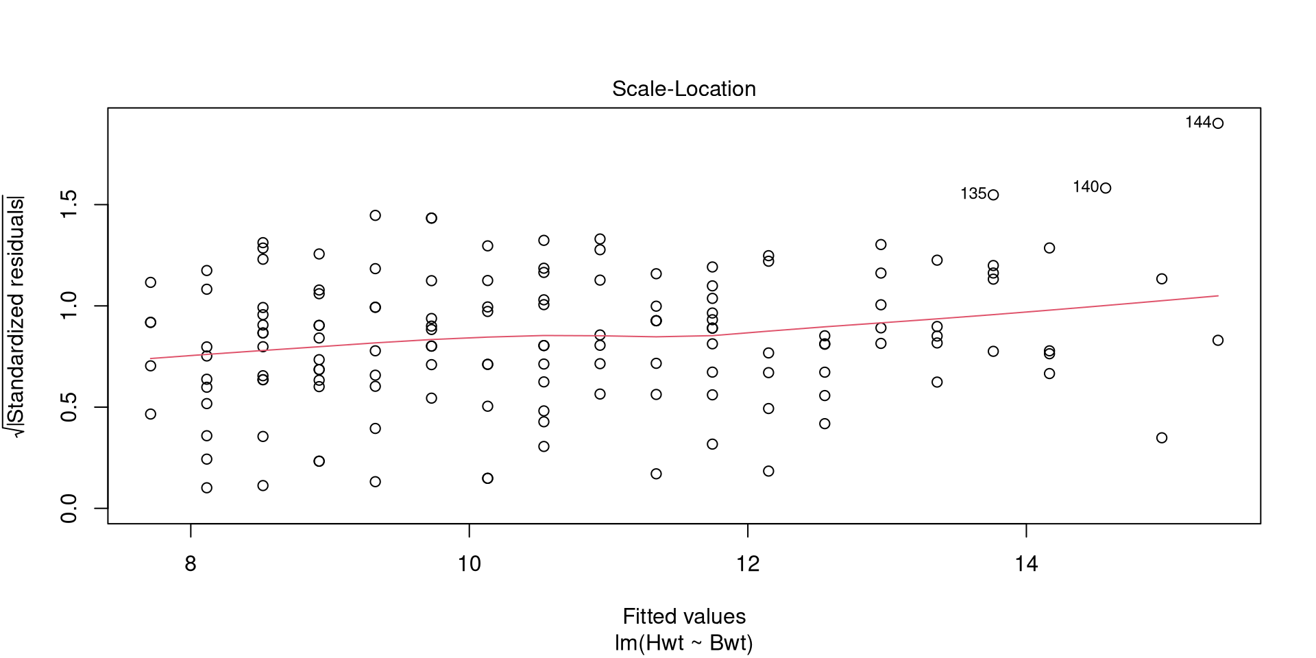
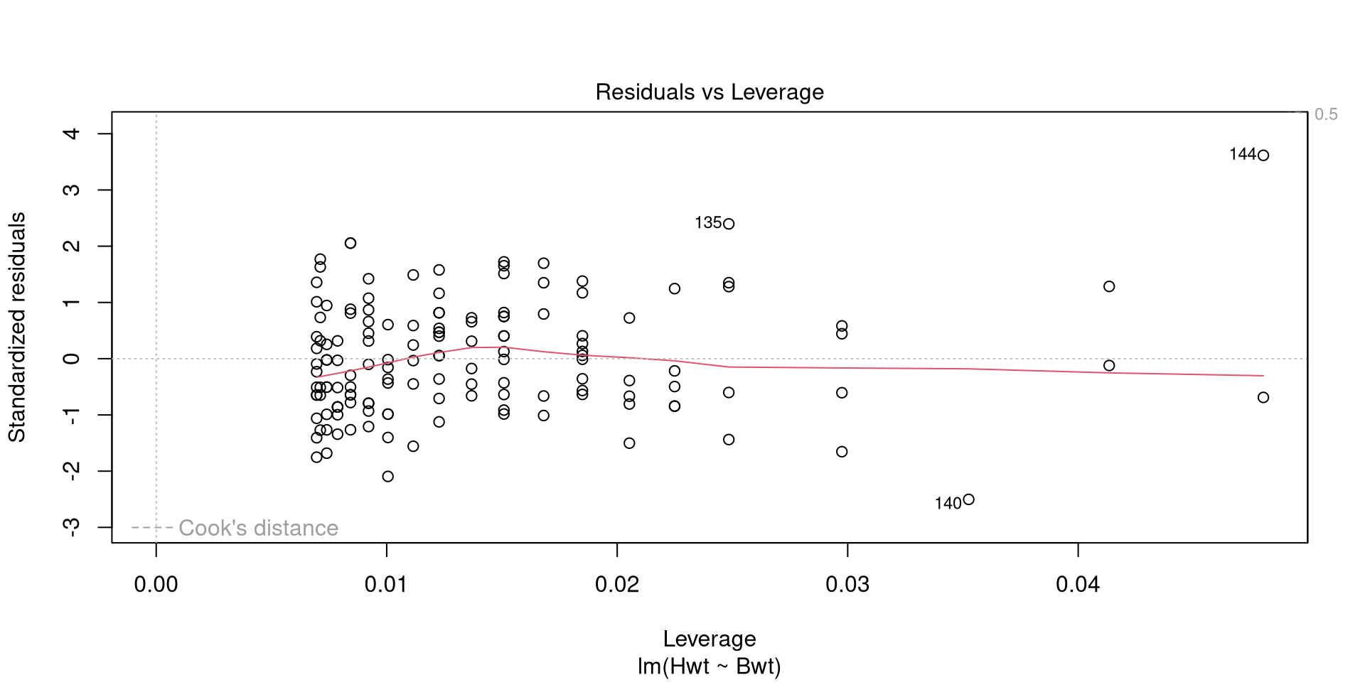
Call:
lm(formula = Hwt ~ Bwt, data = cats)

Coefficients:
(Intercept)          Bwt  
    -0.3567       4.0341

Function summary()

The output of summary() provides an overview on the model:

model <- lm(Hwt ~ Bwt,data=cats)
summary(model)


Call:
lm(formula = Hwt ~ Bwt, data = cats)

Residuals:
    Min      1Q  Median      3Q     Max 
-3.5694 -0.9634 -0.0921  1.0426  5.1238 

Coefficients:
            Estimate Std. Error t value Pr(>|t|)    
(Intercept)  -0.3567     0.6923  -0.515    0.607    
Bwt           4.0341     0.2503  16.119   <2e-16 ***
---
Signif. codes:  0 '***' 0.001 '**' 0.01 '*' 0.05 '.' 0.1 ' ' 1

Residual standard error: 1.452 on 142 degrees of freedom
Multiple R-squared:  0.6466,    Adjusted R-squared:  0.6441 
F-statistic: 259.8 on 1 and 142 DF,  p-value: < 2.2e-16

Plot regression

Plot the regression line

plot(cats$Bwt, cats$Hwt, xlab="Body Weight (kg)",
        ylab="Heart Weight (g)",
         main="Heart Weight vs. Body Weight of Cats")
yhat <- coef(model)[1] + coef(model)[2]*cats$Bwt

lines(x=cats$Bwt,y=yhat,col=2)

Regression line in ggplot

library(ggplot2)
ggplot(cats, aes(Bwt, Hwt))+
  geom_point()+
  geom_smooth(method="lm")+
  xlab("Body Weight (kg)")+
  ylab("Heart Weight (g)")+
  ggtitle("Heart Weight vs. Body Weight of Cats")

Graphical diagnosis

Check residuals directly on plots or use the function plot() function on regression object for diagnosis graphics:

plot(yhat,residuals(model))

qqnorm(residuals(model))
qqline(residuals(model))

plot(model)

Model selection

In R there are pre-built functions which perform automatic model selection, for example, stepAIC() in the package MASS

stepAIC(object, scope, scale = 0, direction = c("both", "backward", "forward"), trace = 1, keep = NULL, steps = 1000, k = 2, ...);

By default, it uses AIC as stopping criterion (argument k=2)
setting k=log(n) we can use BIC. Example:

library(MASS)
model <- lm(Hwt ~ Bwt+Sex,data=cats)
model.new<-stepAIC(model)

Start:  AIC=111.39
Hwt ~ Bwt + Sex

       Df Sum of Sq    RSS    AIC
- Sex   1      0.15 299.53 109.47
<none>              299.38 111.39
- Bwt   1    405.88 705.26 232.78

Step:  AIC=109.47
Hwt ~ Bwt

       Df Sum of Sq    RSS    AIC
<none>              299.53 109.47
- Bwt   1    548.09 847.63 257.26

Prediction

The function predict() computes the predicted value of the response for a new observation.

predict(object, newdata, se.fit = FALSE, interval = c("none", "confidence", "prediction"), level = 0.95, type = c("response", "terms"), ...)

In particular:

object must be replaced by the model fit on the data
newdata must be a data.frame with the new observation(s)
se.fit allows the computation of the standard error
setting interval="prediction", we can compute the prediction interval, with level (default level = 0.95);

Example:

model <- lm(Hwt ~ Bwt,data=cats)
y.hat <- predict(model, newdata = cats, interval="prediction")
predict(model) == coef(model)[1] + coef(model)[2]*cats$Bwt

Exercises 5 Task 1

Logistic regression

Logistic model

\(logit(\pi)=\beta_0+\beta_1 * X_1+ \beta_2 * X_2+...\) ,with \(\pi=Pr(Y=1|X)\)

is a special case of generalized linear model

glm(formula, family = gaussian, data, ...)

to fit a logistic model, the argument family must be set equal to binomial.