Normal Distribution

Mathematical notation

\[ f(x; \mu, \sigma) = \frac{1}{\sigma \sqrt{2\pi}} e^{-\frac{(x - \mu)^2}{2\sigma^2}} \]

Where:

\(x\) is the random variable.
\(\mu\) is the mean of the distribution.
\(\sigma\) is the standard deviation of the distribution.

Sample from Normal Distribution

generate a sample from a Gaussian distribution:

rnorm(n, mean = 0, sd = 1)

Example:

y <- rnorm(n = 100000, mean = 5, sd = sqrt(2))
hist(y, freq = F, ylim = c(0, 0.3))
curve(dnorm(x, mean = 5, sd = sqrt(2)), col = 2, add = T)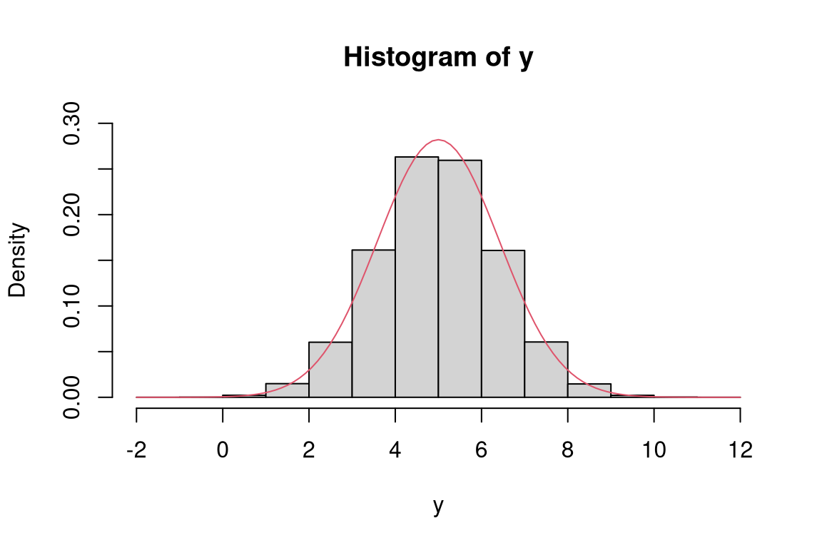

Density function (pdf) of Normal Distribution

Calculate pdf of Normal distribution:

dnorm(x, mean = 0, sd = 1)

y <- rnorm(n = 100000, mean = 0,sd = 1)
hist(y, freq=F, ylim = c(0, 0.4),breaks = 100)
dnorm(-1)
hist(y, freq = F, ylim = c(0, 0.4), breaks = 100)
abline(v = -1, lty = 2)
abline(h = dnorm(-1), lty=2)

[1] 0.2419707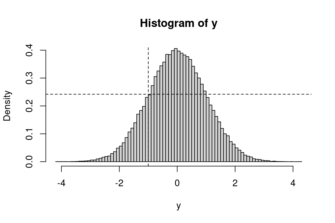

Cumullative Density function (cdf) of Normal Distribution

Calculate pdf of Normal distribution:

pnorm(q, mean = 0, sd = 1)

library(tigerstats)

pnorm(-1)
pnormGC(-1, region = "below", graph = T)

[1] 0.1586553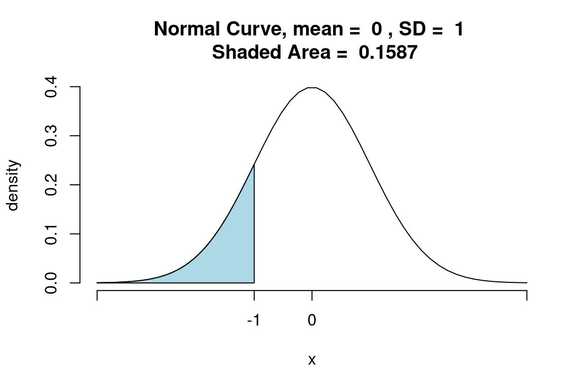

[1] 0.1586553

Cumullative Density function (cdf) of Normal Distribution

library(tigerstats)

plot(ecdf(y),main = "Empirical Cumulative Distribution Function")
abline(v= quantile(ecdf(y),0.158655254), lty = 2)
abline(h= pnorm(-1), lty = 2)
text(x = -0.15, y = 0.2,labels = "(-1,0.159)")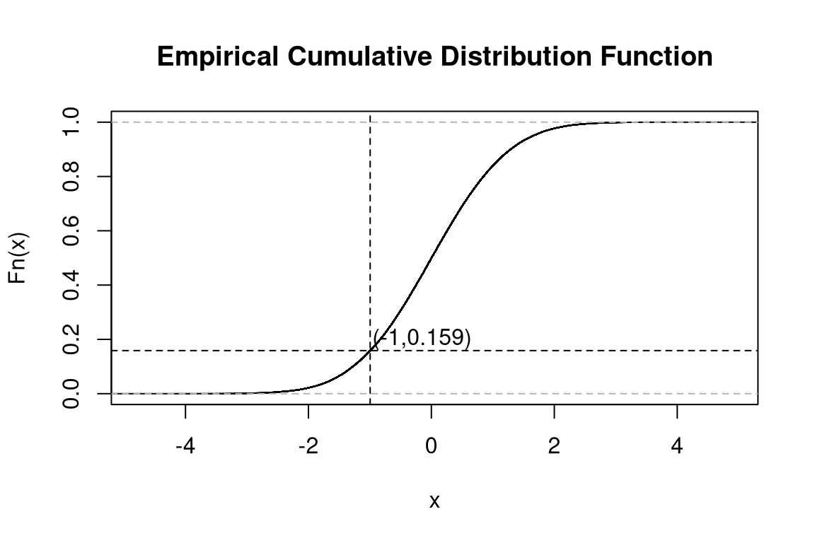

Quantiles of Normal Distribution

qnorm(p, mean = 0, sd = 1)

qnorm(0.158655254)
quantile(ecdf(y),0.158655254)
plot(ecdf(y), main = "Empirical Cumulative Distribution Function")
abline(v = quantile(ecdf(y), 0.158655254), lty = 2)
abline(h = pnorm(-1), lty = 2)
text(x = -0.15, y = 0.2,labels = "(-1,0.159)")

[1] -1

 15.86553% 
-0.9955969

EXAMPLES

Consider \(X \sim N(0,1)\). It is very easy to compute the following probabilities with R:

\(P(X \le 0.89)\)

pnorm(0.89)

[1] 0.8132671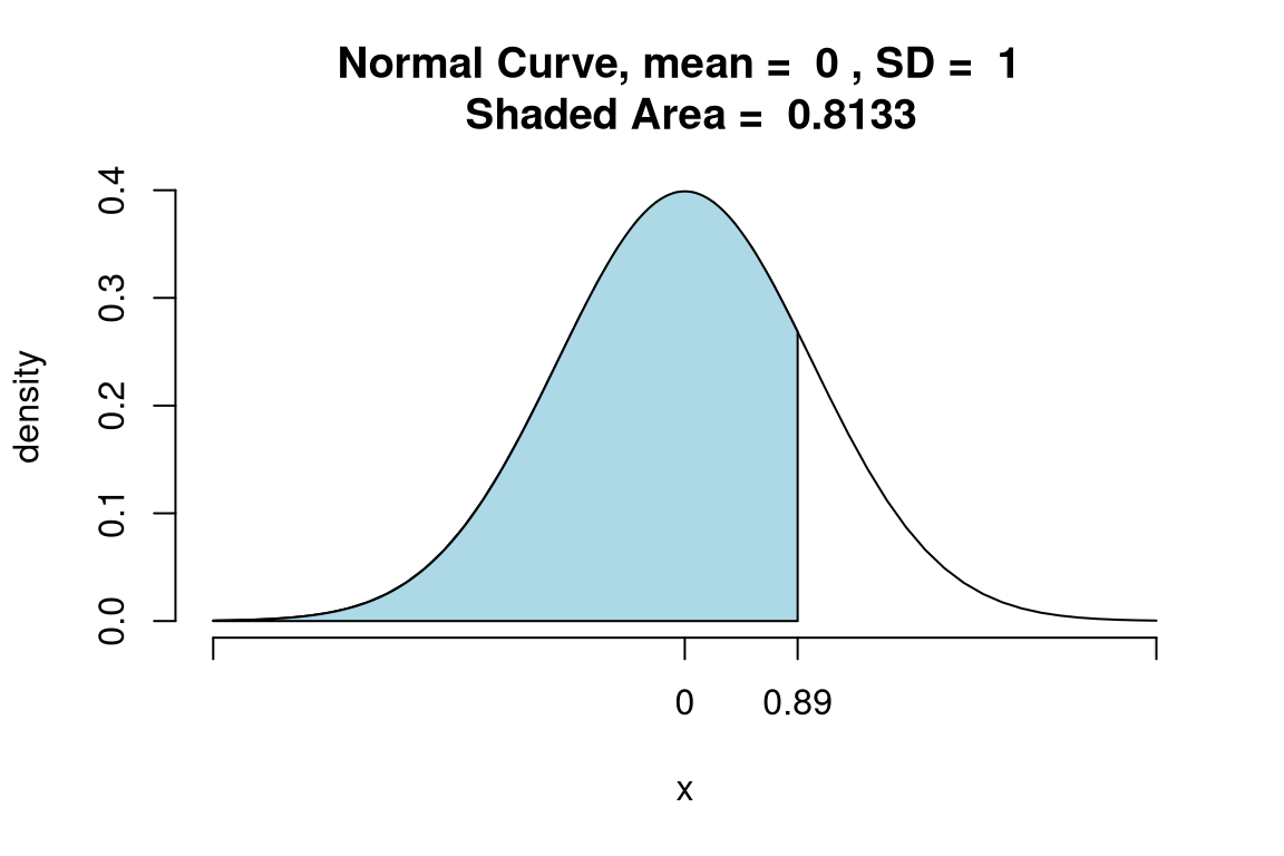

pnormGC(0.89, region="below",graph=T)

[1] 0.8132671

\(P(X \ge 1.21)\)

#| fig-align: "center"
#| layout: [[100]]

1-pnorm(1.21)

[1] 0.1131394

pnormGC(1.21, region="above",graph=T)

[1] 0.1131394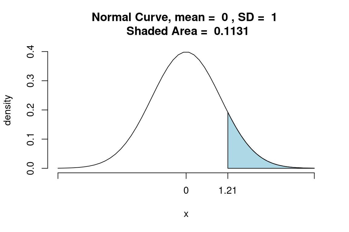

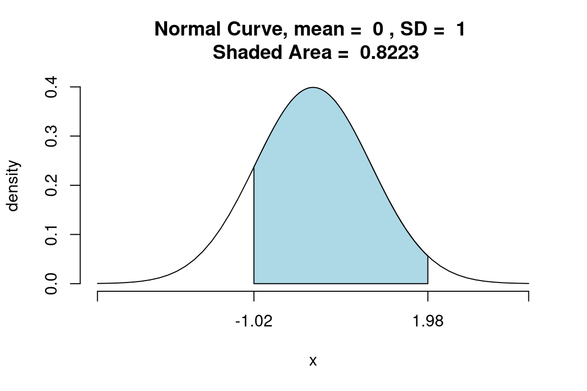
\(P(-1.02 \le X \le 1.98)\)

pnorm(1.98)-pnorm(-1.02)

[1] 0.822284

pnormGC(c(-1.02,1.98), region="between",graph=T)

[1] 0.822284

\(P(\mid X \mid \le 0.92)\)

pnorm(0.92)-pnorm(-0.92)
pnormGC(c(-0.92,0.92), region="between",graph=T)

[1] 0.6424272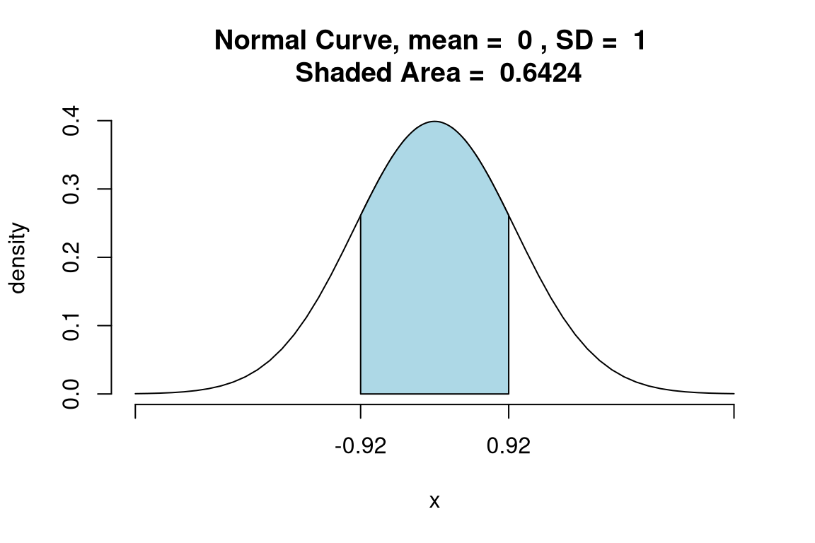

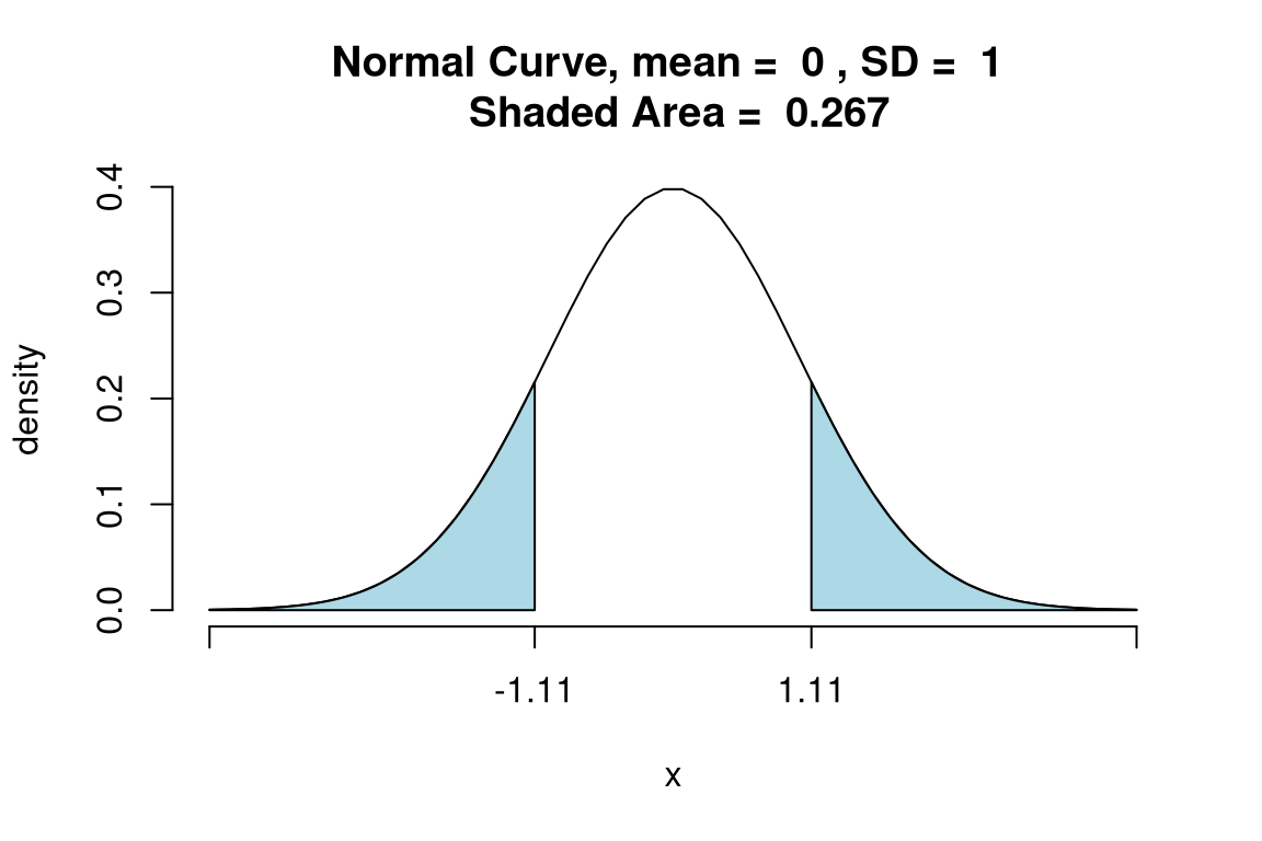
[1] 0.6424272

\(P(\mid X \mid \ge 1.11)\)

(1-pnorm(1.11))+pnorm(-1.11)

[1] 0.266999

pnormGC(c(-1.11,1.11), region="outside",graph=T)

[1] 0.266999

OTHER DISTRIBUTIONS

We can use other distributions like the Normal distribution, for example - binomial: rbinom, dbinom, pbinom, qbinom

uniform: runif, dunif, punif, qunif
Student’s t: rt, dt, pt, qt
…