Tests in R

Raphael Rehms und Jonathan Christ

Tests in R

Prelude

CONFIDENCE INTERVALS

• it is an interval estimate;

• we construct an interval following a procedure that, if applied in a large number of replications of the experiment, gives intervals which contain the true value \(1 - \alpha\) of the time;

• \(1 - \alpha\) is called confidence level;

• usual values are 0.90, 0.95 and 0.99.

EXAMPLES of CONFIDENCE INTERVALS

• true mean, gaussian distribution, known variance:

x <- rnorm(100,mean=1,sd=2)
mean.x <- mean(x)
low <- mean.x - qnorm(0.975)*2/sqrt(100)
up <- mean.x + qnorm(0.975)*2/sqrt(100)
c(low,up)

[1] 0.6694404 1.4534260

• true mean, gaussian distribution, unknown variance:

sd.x <- sd(x)
low <- mean.x - qt(0.975, df=99)*sd.x/sqrt(100)
up <- mean.x + qt(0.975, df=99)*sd.x/sqrt(100)
c(low,up)

[1] 0.7004186 1.4224477

Excercise 4 Task 3

STUDENT’S ONE-SAMPLE TEST

• \(H_0 : \mu = \mu_0\)

• \(H_1 :\mu \neq \mu_0\)

t.test(x, mu=\(\mu_0\), alternative='two-sided')

t.test(x, mu=\(\mu_0\), alternative='greater')

t.test(x, mu=\(\mu_0\), alternative='less')

• default alternative is ‘two-sided’

x <- rnorm(100, mean=3, sd=1)
t.test(x, mu=1)

    One Sample t-test

data:  x
t = 19.082, df = 99, p-value < 2.2e-16
alternative hypothesis: true mean is not equal to 1
95 percent confidence interval:
 2.804082 3.222809
sample estimates:
mean of x 
 3.013445 

Further examples

Further examples: greater, less

t.test(x, mu=1, alternative="greater")

    One Sample t-test

data:  x
t = 19.082, df = 99, p-value < 2.2e-16
alternative hypothesis: true mean is greater than 1
95 percent confidence interval:
 2.83825     Inf
sample estimates:
mean of x 
 3.013445 

t.test(x, mu=1, alternative="less")

    One Sample t-test

data:  x
t = 19.082, df = 99, p-value = 1
alternative hypothesis: true mean is less than 1
95 percent confidence interval:
    -Inf 3.18864
sample estimates:
mean of x 
 3.013445 

TWO-SAMPLE T-TEST (UNEQUAL VARIANCE)

• \(Var[X] \neq Var[Y]\)

• \(H_0: \mu_X = \mu_Y\)

t.test(x, y, alternative=c('two.sided', 'less','greater'))

Example:

x <- rnorm(100, mean=4, sd=5)
y <- rnorm(100, mean=2, sd=2)
t.test(x, y)

    Welch Two Sample t-test

data:  x and y
t = 2.5924, df = 128.19, p-value = 0.01064
alternative hypothesis: true difference in means is not equal to 0
95 percent confidence interval:
 0.3542169 2.6379177
sample estimates:
mean of x mean of y 
 3.621649  2.125582 

TWO-SAMPLE T-TEST (EQUAL VARIANCE)

• \(Var[X] = Var[Y]\)

• \(H_0: \mu_X = \mu_Y\)

t.test(x, y, var.equal=T,alternative=c('two.sided', 'less', 'greater'))

Example:

x <- rnorm(100, mean=4, sd=1)
y <- rnorm(100, mean=2, sd=1)
t.test(x, y, var.equal=T)

    Two Sample t-test

data:  x and y
t = 14.71, df = 198, p-value < 2.2e-16
alternative hypothesis: true difference in means is not equal to 0
95 percent confidence interval:
 1.729849 2.265464
sample estimates:
mean of x mean of y 
 3.902018  1.904362 

F-TEST FOR COMPARING VARIANCES

• \(H_0: \sigma^2_X = \sigma^2_Y\)

• \(H_1: \sigma^2_X \neq \sigma^2_Y\)

var.test(x, y, ratio = 1,alternative=c('two.sided', 'less', 'greater'),conf.level = 0.95)

Example:

x <- rnorm(80, mean=4, sd=5)
y <- rnorm(20, mean=2, sd=2)
var.test(x, y)

    F test to compare two variances

data:  x and y
F = 9.3231, num df = 79, denom df = 19, p-value = 1.776e-06
alternative hypothesis: true ratio of variances is not equal to 1
95 percent confidence interval:
  4.165734 17.769619
sample estimates:
ratio of variances 
          9.323063 

PROPORTION TEST 1

• \(H_0: p = p_0\)

• \(H_1: p \neq p_0\)

prop.test(x, n, p)

• x: number of successes

• n: total number of trials

• p: proportion to be tested.

• Example:

# Load preprocessed version of the data saved as .RData file
load(file="myNhanes.RData")
prop.test(sum(mydata$male), length(mydata$male), p=0.5)

    1-sample proportions test with continuity correction

data:  sum(mydata$male) out of length(mydata$male), null probability 0.5
X-squared = 0.2738, df = 1, p-value = 0.6008
alternative hypothesis: true p is not equal to 0.5
95 percent confidence interval:
 0.4898438 0.5177503
sample estimates:
     p 
0.5038 

PROPORTION TEST 2

• \(H_0: p_1 = p_2\)

• \(H_1: p_1 \neq p_2\)

prop.test(table(x, y))

• x: first (categorical) variable

• y second (binary) variable

• Example:

# prop.test(table(educ, male))
tbl <- table(mydata$educ, mydata$male)
prop.test(tbl)

    5-sample test for equality of proportions without continuity correction

data:  tbl
X-squared = 13.481, df = 4, p-value = 0.00915
alternative hypothesis: two.sided
sample estimates:
   prop 1    prop 2    prop 3    prop 4    prop 5 
0.5218295 0.5082707 0.5292929 0.4605078 0.4881356 

Quick Summary

t.test(height[male==T],height[male==F])

var.test(height[male==T],height[male==F])

• and a Z-test, testing the equality of proportions:

table(male,heartdis_ever,dnn=c("Male","Heart disease"))
prop.table(table(male,!heartdis_ever,dnn=c("Male","Heart disease")),1)
prop.test(table(male,!heartdis_ever))

Chi-Square test

• \(H_0: \pi_1 = \pi_2 = \pi\)

chisq.test(x, y = NULL, correct = TRUE, p =rep(1/length(x), length(x)), rescale.p = FALSE,
           simulate.p.value = FALSE, B = 2000)

• you can pass to the function:
  • a contingency table;
  • directly two categorical vectors.

Examples:

x <- c("M","F","M","F","M","M","F","F","M")
y <- c("Y","N","N","N","Y","Y","N","Y","N")
chisq.test(x,y)

    Pearson's Chi-squared test with Yates' continuity correction

data:  x and y
X-squared = 0.14062, df = 1, p-value = 0.7077

or, with a contingency table,

tab <- table(x,y)
chisq.test(tab)

    Pearson's Chi-squared test with Yates' continuity correction

data:  tab
X-squared = 0.14062, df = 1, p-value = 0.7077

Fisher test

• exact test

fisher.test(x, y = NULL, workspace = 200000,
    hybrid = FALSE, control = list(), or = 1,
    alternative = "two.sided", conf.int = TRUE,
    conf.level = 0.95, simulate.p.value = FALSE, B =
    2000)

• you can pass to the function two factor vectors

Examples:

fisher.test(x,y)

    Fisher's Exact Test for Count Data

data:  x and y
p-value = 0.5238
alternative hypothesis: true odds ratio is not equal to 1
95 percent confidence interval:
   0.1497998 312.5621395
sample estimates:
odds ratio 
  3.764195 

. . . or a contingency table

tab <- table(x,y)
fisher.test(tab)

    Fisher's Exact Test for Count Data

data:  tab
p-value = 0.5238
alternative hypothesis: true odds ratio is not equal to 1
95 percent confidence interval:
   0.1497998 312.5621395
sample estimates:
odds ratio 
  3.764195 

McNemar test

• symmetry of rows and columns;

mcnemar.test(x, y = NULL, correct = TRUE)

• you can pass to the function two factor vectors

Examples:

mcnemar.test(x,y)

    McNemar's Chi-squared test with continuity correction

data:  x and y
McNemar's chi-squared = 0, df = 1, p-value = 1

. . . or a contingency table

tab <- table(x,y)
mcnemar.test(tab)

    McNemar's Chi-squared test with continuity correction

data:  tab
McNemar's chi-squared = 0, df = 1, p-value = 1

Excercise 4 Task 4

Non-parametric Tests

Sign test

• \(H_0 : median = md_0\)

• we need the package BSDA

SIGN.test(x, y = NULL, md = 0, alternative = "two.sided", conf.level = 0.95)

Example:

library(BSDA)
x <- rpois(100,5)
SIGN.test(x, md=5)

    One-sample Sign-Test

data:  x
s = 38, p-value = 0.3857
alternative hypothesis: true median is not equal to 5
95 percent confidence interval:
 4 5
sample estimates:
median of x 
          5 

Achieved and Interpolated Confidence Intervals: 

                  Conf.Level L.E.pt U.E.pt
Lower Achieved CI     0.9431      4      5
Interpolated CI       0.9500      4      5
Upper Achieved CI     0.9648      4      5

Wilcoxon test

• \(H_0: median = md_0\)

• test based on ranks

wilcox.test(x, y = NULL, alternative = c("two.sided", "less", "greater"), mu = 0,
            paired = FALSE, exact = NULL, correct = TRUE, conf.int = FALSE,
            conf.level = 0.95, ...)

Example:

x <- rpois(100,5)
wilcox.test(x,mu=5)

    Wilcoxon signed rank test with continuity correction

data:  x
V = 1693.5, p-value = 0.8217
alternative hypothesis: true location is not equal to 5

Recall: Sign test vs. Wilcoxon test vs. t-test part 1

Sign test:

• Applicable for ordinal or higher scale level

• No distributional assumptions

• Low power

Wilcoxon test:

• Applicable for discrete or continuous quantitative data

• Symmetrical distribution required

• Intermediate power

T-test:

• Normal distribution required

• Highest power

Compare all tests on the same data (we assume Normal distributed data!)

set.seed(123)
x <- rnorm(20,0.5)
c(
  signTest = BSDA::SIGN.test(x, md = 0)$p.value,
  wilcoxonTest =wilcox.test(x,mu=0)$p.value,
  tTest = t.test(x, mu = 0)$p.value
)

    signTest wilcoxonTest        tTest 
  0.04138947   0.01068878   0.00822065 

Mann-Whitney U test

• \(H_0: median_1 = median_2\)

• non-parametric test for independent samples

• package coin (Why extra package and not using wilcox.test? -> https://stats.stackexchange.com/questions/31417/what-is-the-difference-between-wilcox-test-and-coinwilcox-test-in-r)

wilcox_test(formula, data, subset = NULL, weights= NULL, ...)

• needs a formula, e.g. y~x.

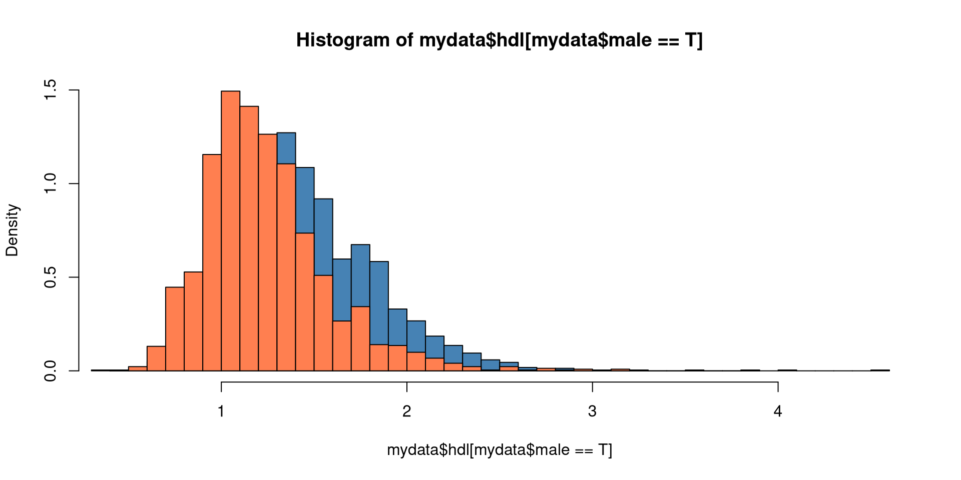
Example hdl in NHANES data (not normal):

hist(mydata$hdl[mydata$male == T], breaks = 40, col = "steelblue", freq = F, ylim=c(0,1.5))
hist(mydata$hdl[mydata$male == F], breaks = 40, col = "coral", add = T, freq = F)

coin::wilcox_test(hdl ~ as.factor(male), data = mydata)

    Asymptotic Wilcoxon-Mann-Whitney Test

data:  hdl by as.factor(male) (FALSE, TRUE)
Z = -21.838, p-value < 2.2e-16
alternative hypothesis: true mu is not equal to 0

wilcox.test(hdl ~ as.factor(male), data = mydata)

    Wilcoxon rank sum test with continuity correction

data:  hdl by as.factor(male)
W = 1520720, p-value < 2.2e-16
alternative hypothesis: true location shift is not equal to 0

Correlation

cor(X,Y)

cor(x, y = NULL, use = "everything", method =c("pearson", "kendall", "spearman"))

• correlation between x and y

• with incomplete observations, we may want to set use =“complete.obs”

• based on the argument method, the function cor() computes

  • Pearson’s r (default)

  • Kendall’s \(\tau\) (rank based)

  • Spearman’s \(\rho\) (rank based)

Example:

x<-rnorm(10)
y<-rnorm(10)
cor(x,y)

[1] -0.4372649

Correlation test

• test for correlation between paired samples

cor.test(x, y, alternative = c("two.sided","less", "greater"), method = c("pearson","kendall", "spearman"), conf.level = 0.95, ...)

• \(H_1\) is defined through the argument alternative

• the argument method sets the correlation coefficient

Example:

cor.test(x,y)

    Pearson's product-moment correlation

data:  x and y
t = -1.3752, df = 8, p-value = 0.2063
alternative hypothesis: true correlation is not equal to 0
95 percent confidence interval:
 -0.8365717  0.2654408
sample estimates:
       cor 
-0.4372649 

Excercise 4 Task 5