dat <- read.csv("NHANES1.csv")

# make factors
integer_info <- sapply(dat, is.integer)
integer_info[which(names(integer_info) == "age")] <- FALSE  # age should stay an integer
dat[integer_info] <- lapply(dat[integer_info], as.factor)Exercise 4: Solutions second part
Load the data in R.
Task 2.1
Plot the variable rr_sys as a function of bmi.
library(ggplot2)
ggplot(dat, aes(rr_sys, bmi))+
  geom_point()
Warning: Removed 498 rows containing missing values or values outside the scale range
(`geom_point()`).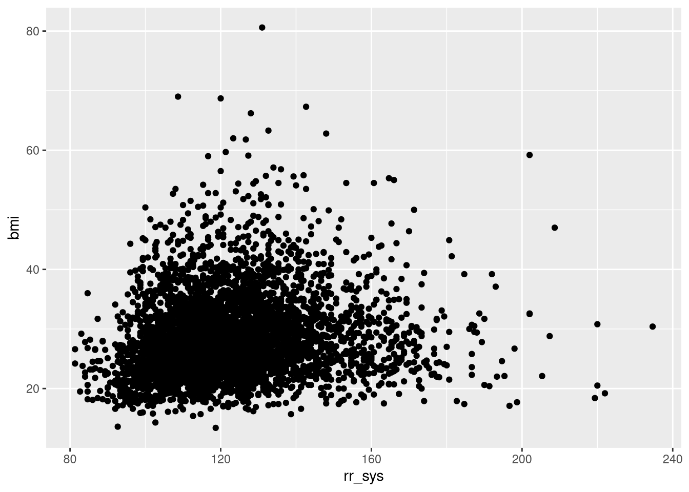
# baseplot
plot(dat$rr_sys, dat$bmi)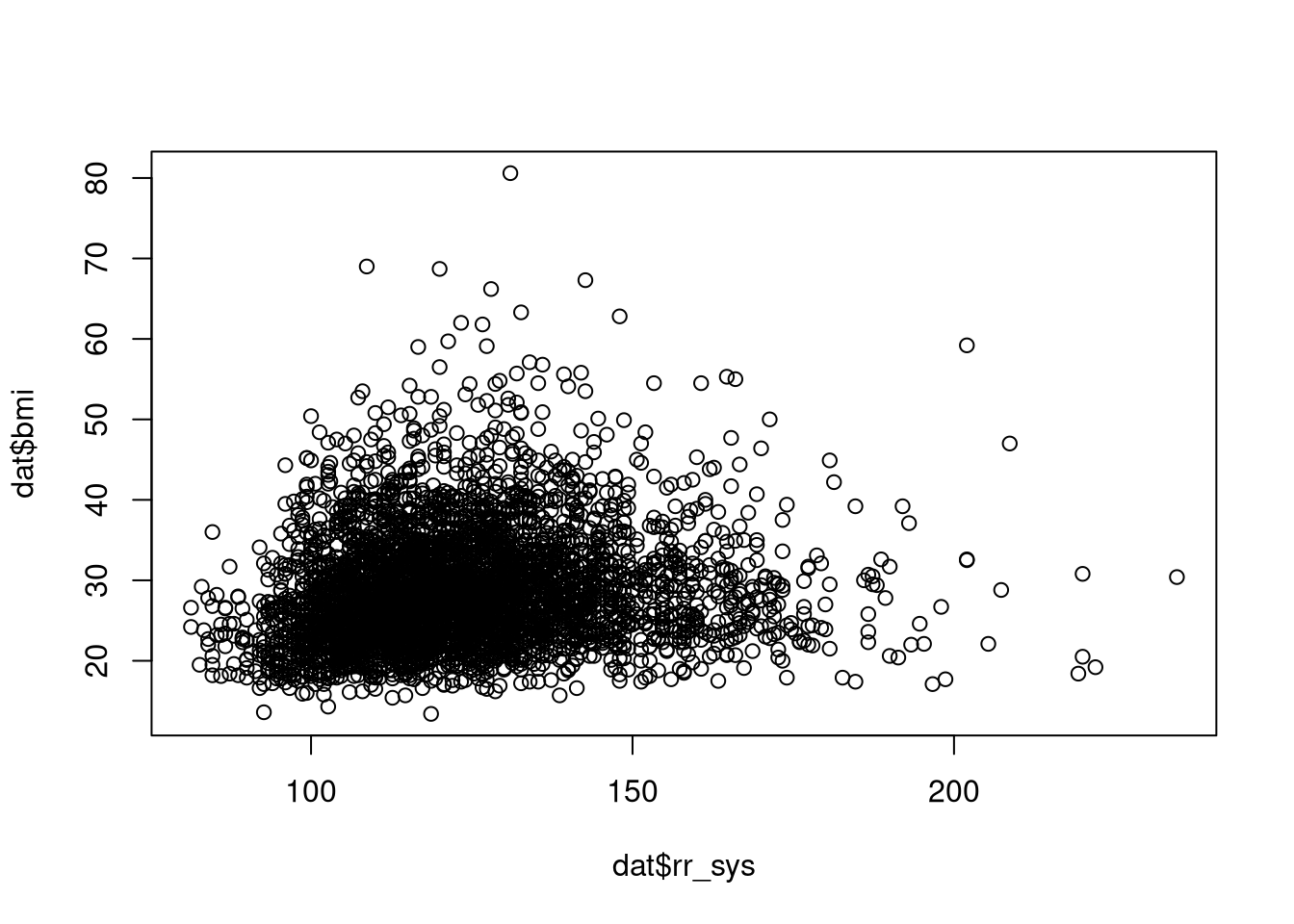
Task 2.2
Now we want to plot the variable rr_sys against diab_lft. Which plot should we use here?
ggplot(dat, aes(diab_lft, rr_sys))+
  geom_boxplot()
Warning: Removed 437 rows containing non-finite outside the scale range
(`stat_boxplot()`).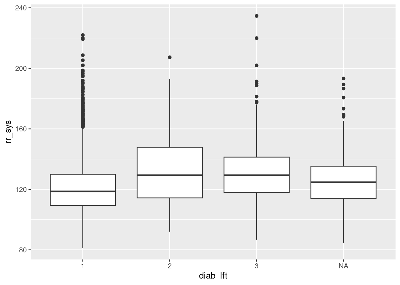
# baseplot
boxplot(rr_sys~diab_lft, names=c("None", "Prediabetes", "Diabetes"), data = dat)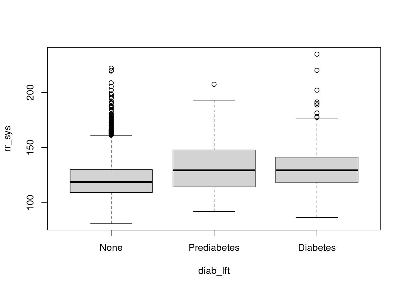
Task 2.3
Plot the BMI against educ and give a short interpretation.
ggplot(dat, aes(educ, bmi))+
  geom_boxplot()
Warning: Removed 290 rows containing non-finite outside the scale range
(`stat_boxplot()`).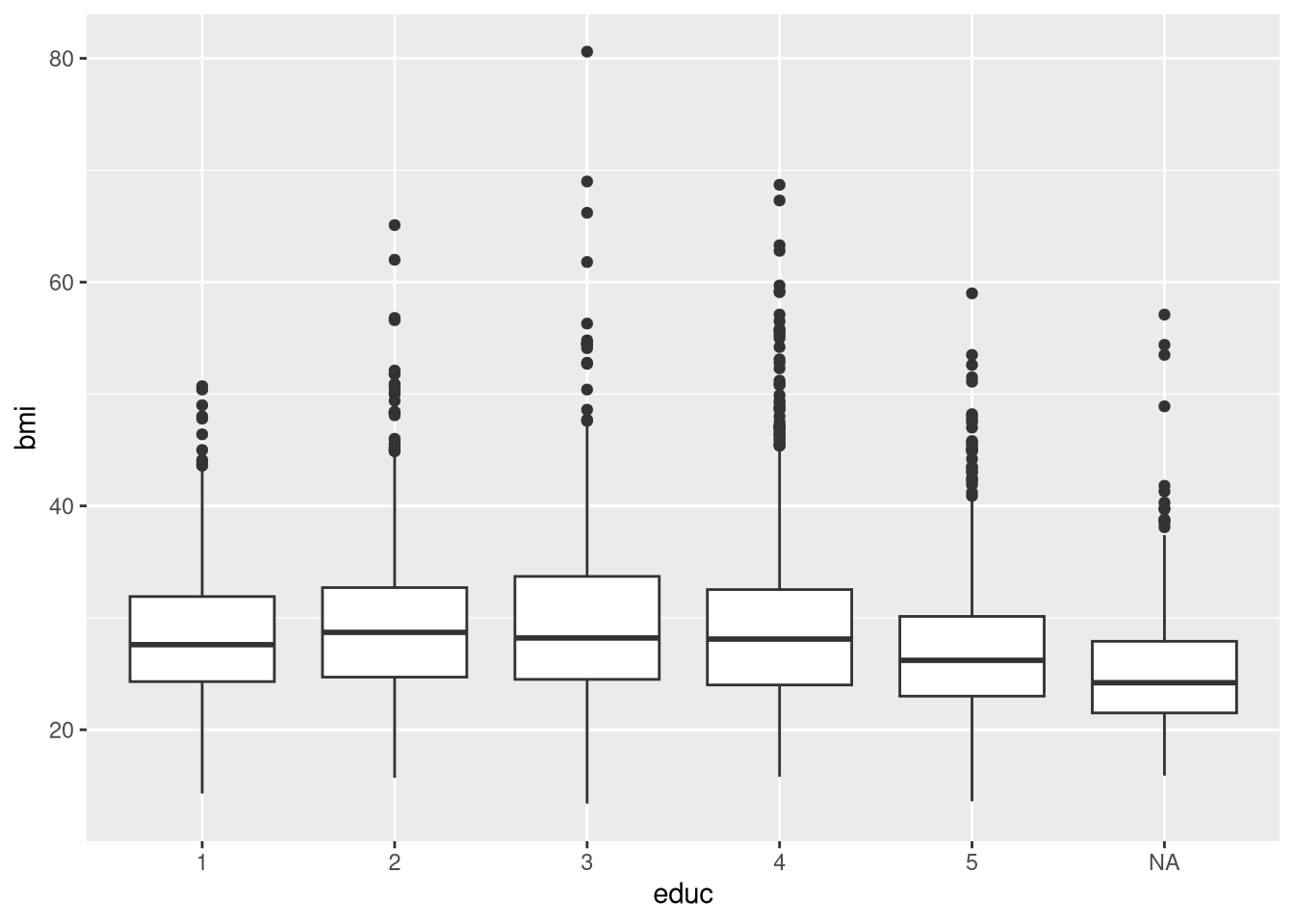
# baseplot
boxplot(bmi~educ, data = dat)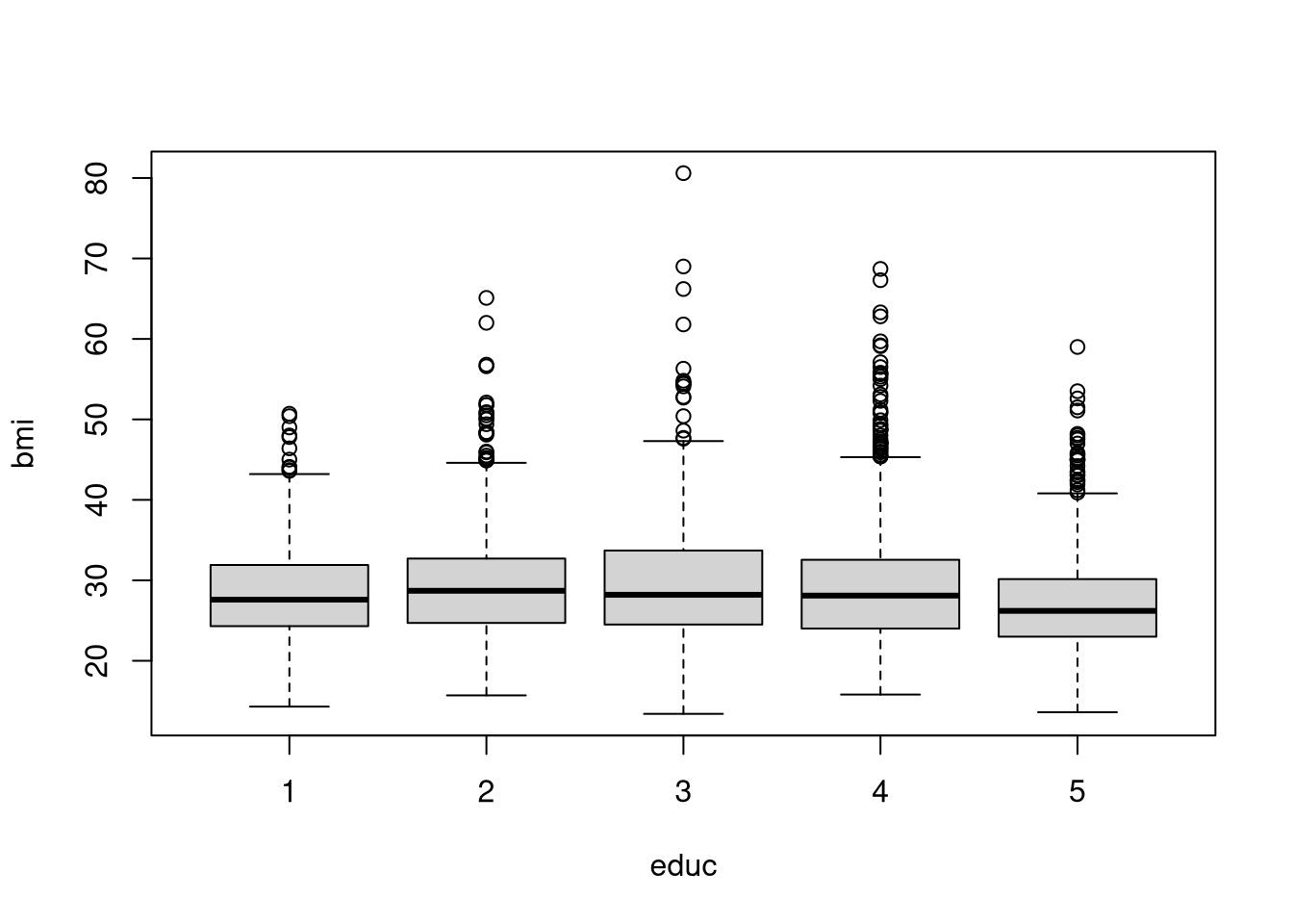
Task 2.4
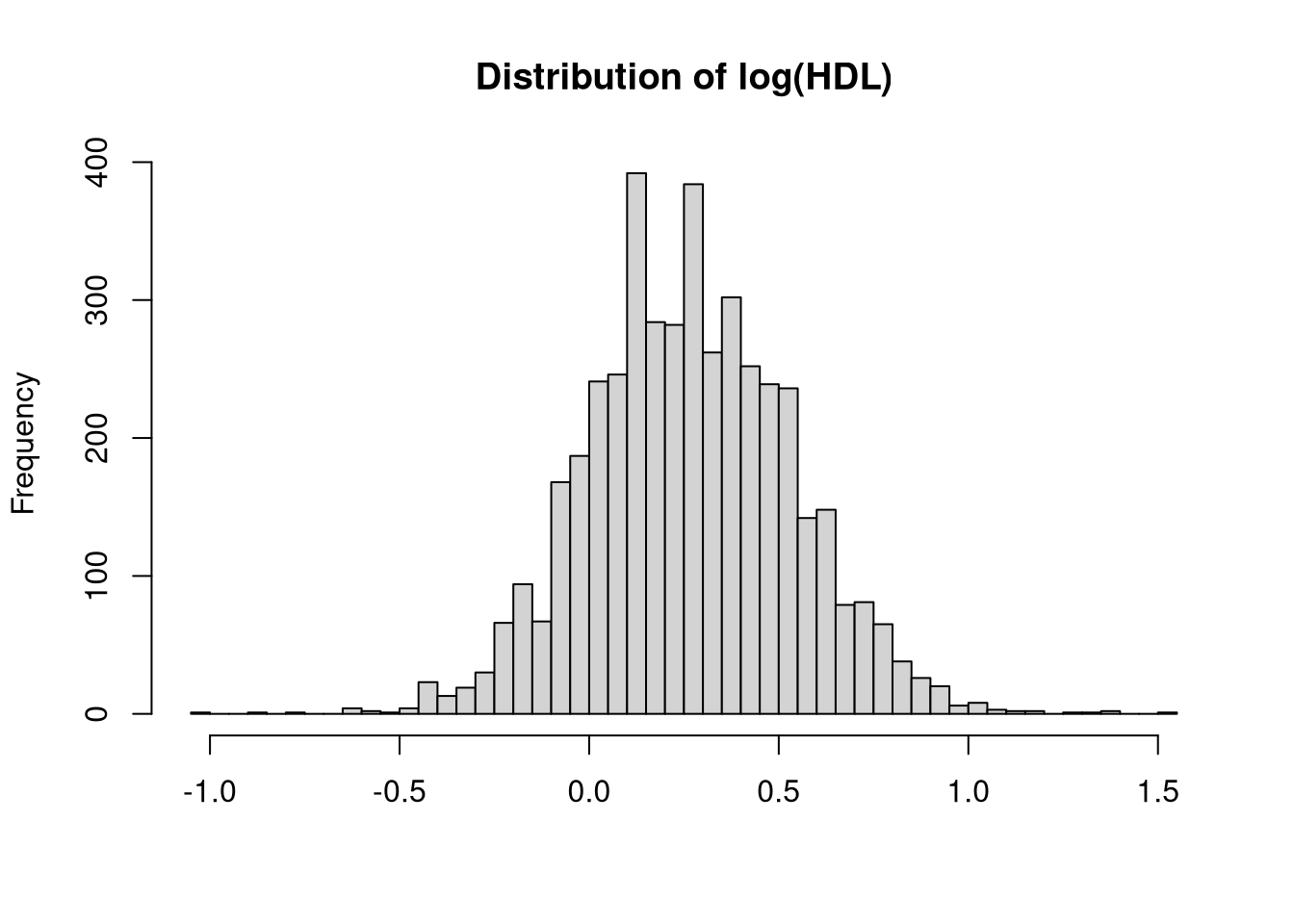
Plot the histogram of the high-density lipoprotein (HDL) cholesterol levels. How does the distribution of HDL look like?
ggplot(dat, aes(hdl))+
  geom_histogram(bins=50)
Warning: Removed 574 rows containing non-finite outside the scale range
(`stat_bin()`).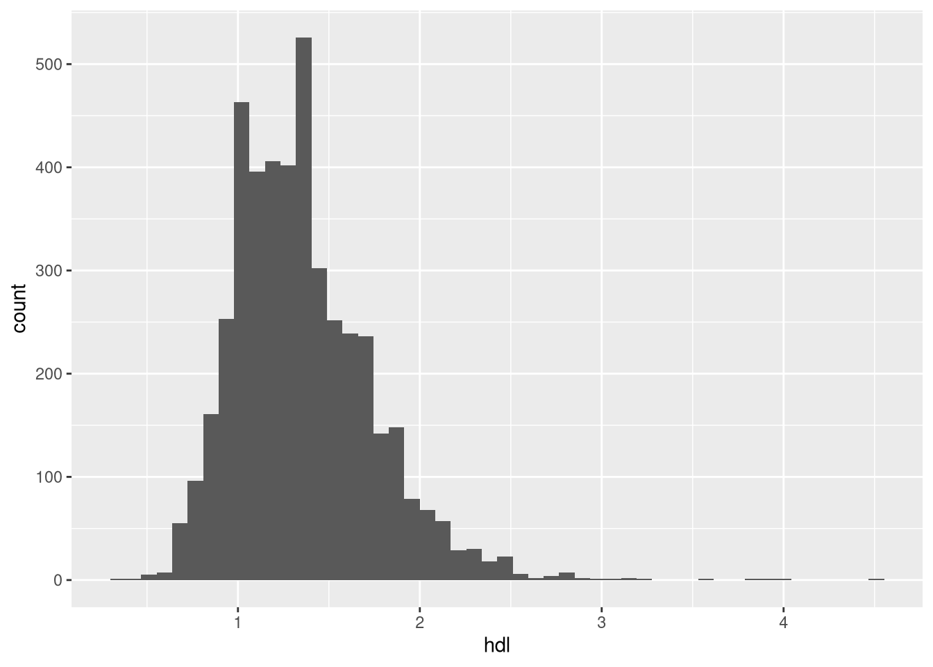
# baseplot
hist(dat$hdl, breaks=50)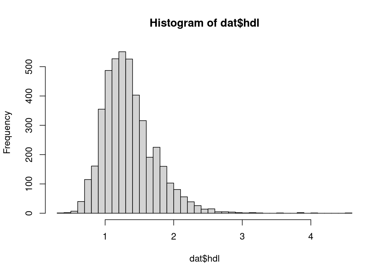
Task 2.5
Can you convert the variable HDL so that its distribution looks more normal? Create such a variable and add it to your data set.
dat$logHDL <- log(dat$hdl)

ggplot(dat, aes(logHDL))+
  geom_histogram(bins=50)
Warning: Removed 574 rows containing non-finite outside the scale range
(`stat_bin()`).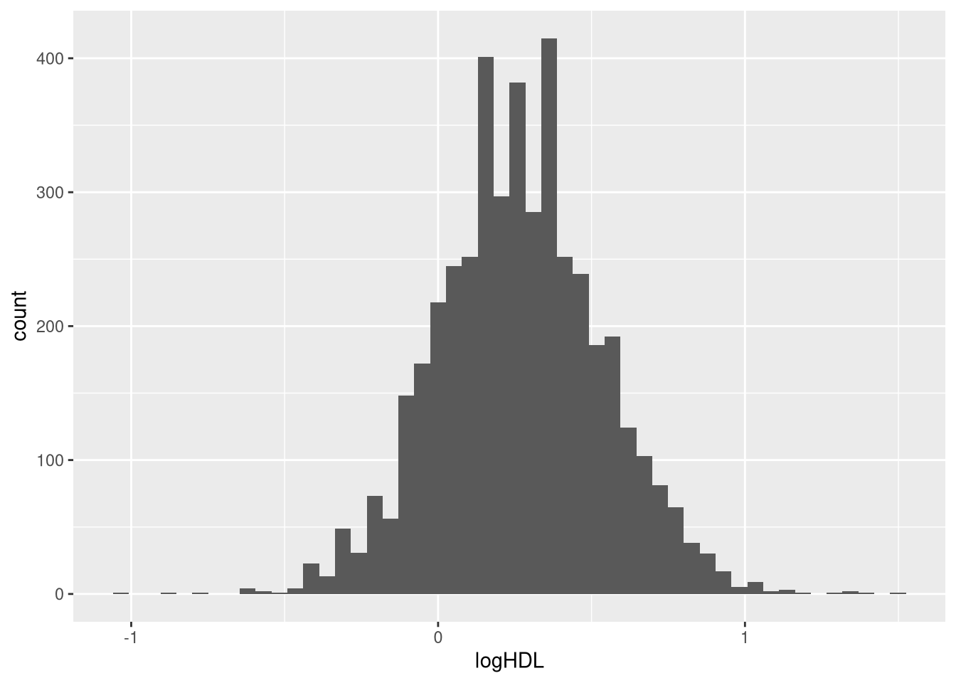
hist(dat$logHDL, breaks=50, main="Distribution of log(HDL)", xlab="")