Exercise 4: Solutions third part

Load the data in R.

dat <- read.csv("NHANES1.csv")

# make factors
integer_info <- sapply(dat, is.integer)
integer_info[which(names(integer_info) == "age")] <- FALSE  # age should stay an integer
dat[integer_info] <- lapply(dat[integer_info], as.factor)

Task 3.1

Is the variable height normally distributed in males and females? Check this by analyzing graphically the two sub-samples.

hist(dat$height[dat$male==T],breaks=50)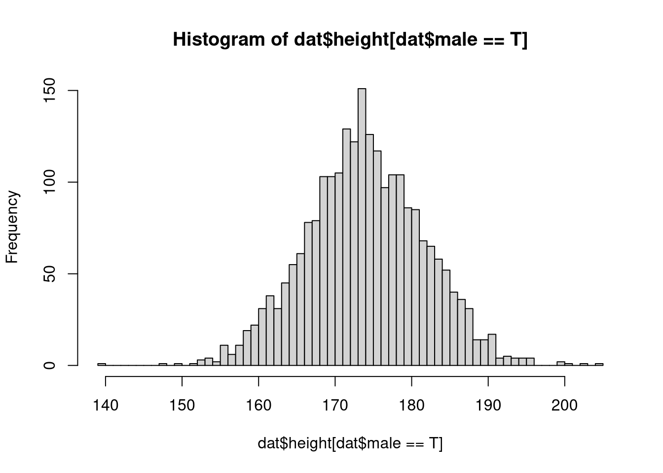

hist(dat$height[dat$male==F],breaks=50)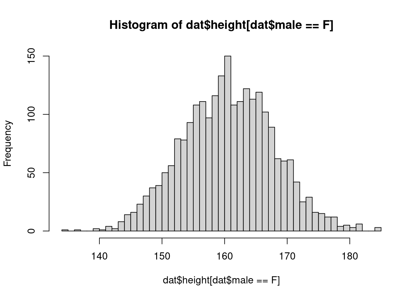

# diagonal line , all points should lie on that line
qqnorm(dat$height[dat$male==T])
qqline(dat$height[dat$male==T])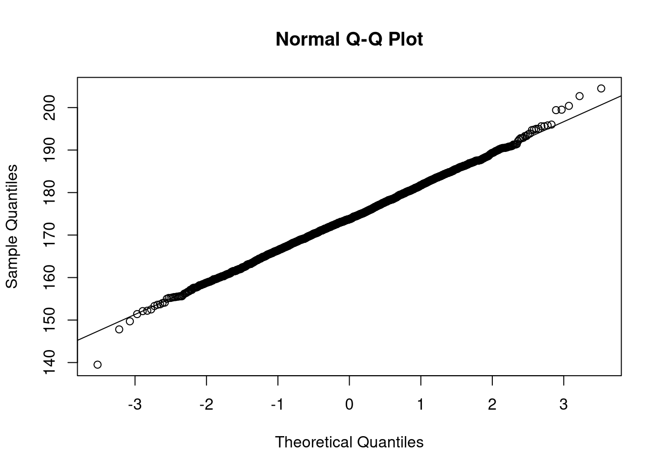

qqnorm(dat$height[dat$male==F])
qqline(dat$height[dat$male==F])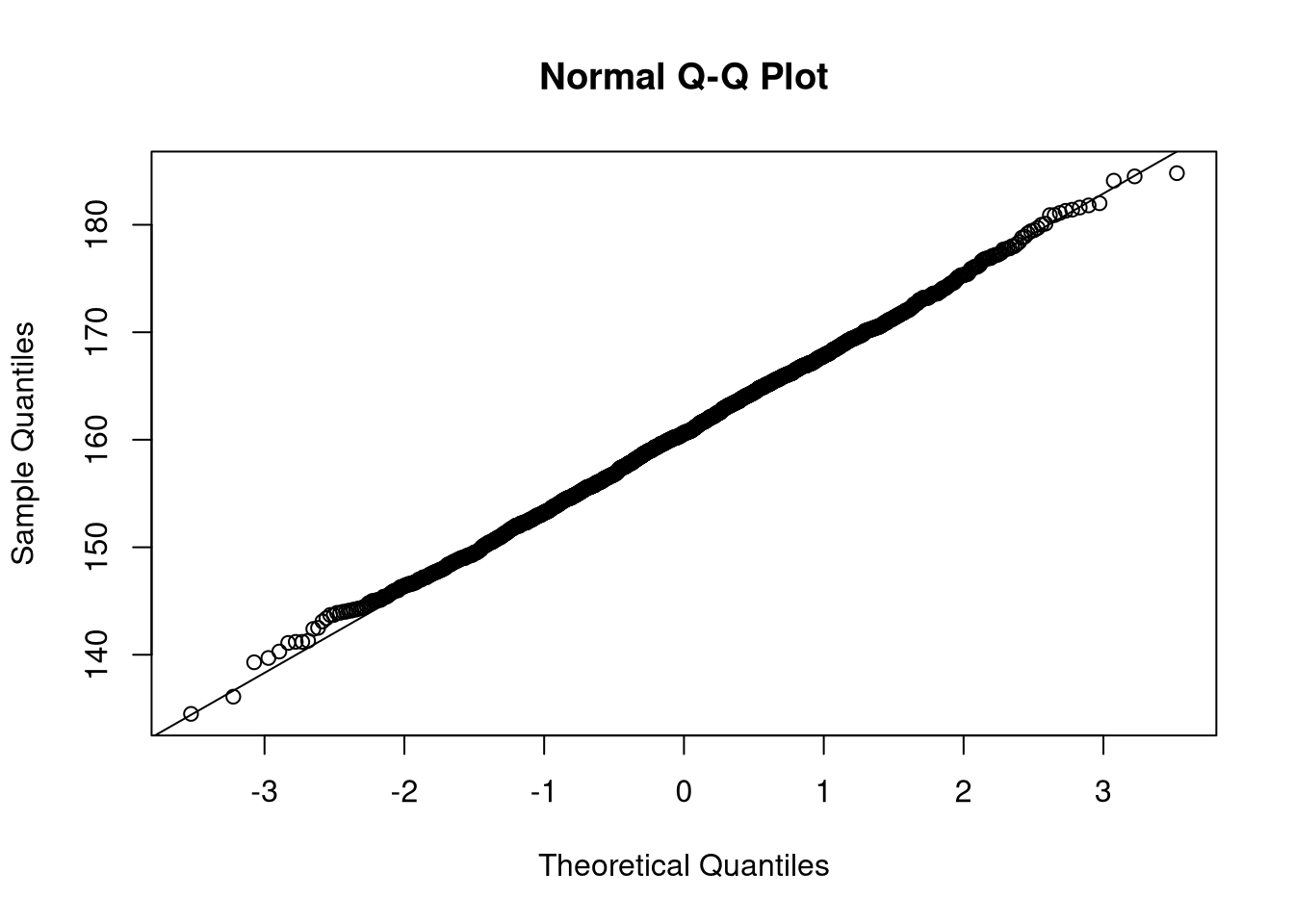

Task 3.2

Suppose that the value of the variance for the male height is known and equal to 64. Construct a 95% confidence interval for the mean.

low <- mean(dat$height[dat$male],na.rm=T) - qnorm(0.975)*sqrt(64/(length(dat$height[dat$male])-sum(is.na(dat$height[dat$male]))))
up <- mean(dat$height[dat$male],na.rm=T) + qnorm(0.975)*sqrt(64/(length(dat$height[dat$male])-sum(is.na(dat$height[dat$male]))))
c(low,up)

[1] 173.6484 174.2949

Task 3.3

Repeat the procedure for the female population, with unknown variance and using a confidence level of 90%.

low <- mean(dat$height[!dat$male],na.rm=T) - qnorm(0.95)*sqrt(64/(length(dat$height[!dat$male])-sum(is.na(dat$height[!dat$male]))))
up<- mean(dat$height[!dat$male],na.rm=T) + qnorm(0.95)*sqrt(64/(length(dat$height[!dat$male])-sum(is.na(dat$height[!dat$male]))))
c(low,up)

[1] 160.3792 160.9201