dat <- read.csv("NHANES1.csv")

# make factors
integer_info <- sapply(dat, is.integer)
integer_info[which(names(integer_info) == "age")] <- FALSE  # age should stay an integer
dat[integer_info] <- lapply(dat[integer_info], as.factor)Exercise 4: Solutions 5th part
Load the data in R.
Task 4.1
Use a chi-square test in order to test whether the presence of chronic bronchitis and the current smoking status are independent.
table(dat$cbronch_now, dat$smokstat)
         1  2  3
  FALSE 37  8 28
TRUE 32 3 43chisq.test(dat$cbronch_now, dat$smokstat)
    Pearson's Chi-squared test

data:  dat$cbronch_now and dat$smokstat
X-squared = 5.6447, df = 2, p-value = 0.05947
Task 4.2
Use a Fisher test to verify the independence between sex and the presence of any kind of liver disease.
table(dat$livdis_now, dat$male)
        FALSE TRUE
  FALSE    33   38
TRUE 50 60fisher.test(dat$livdis_now, dat$male)
    Fisher's Exact Test for Count Data

data:  dat$livdis_now and dat$male
p-value = 1
alternative hypothesis: true odds ratio is not equal to 1
95 percent confidence interval:
 0.547707 1.979023
sample estimates:
odds ratio
  1.041893
Task 4.3
Perform a sign test both on hdl and on log-hdl to test the hypothesis that the median of the cholesterol level is 1.30. Is the median significantly different from 1.30? Do you obtain the same results using hdl and logHdl?
library(BSDA)Loading required package: lattice
Attaching package: 'BSDA'The following object is masked from 'package:datasets':
OrangeSIGN.test(dat$hdl, md = 1.30)
    One-sample Sign-Test

data:  dat$hdl
s = 2180, p-value = 0.3286
alternative hypothesis: true median is not equal to 1.3
95 percent confidence interval:
 1.29 1.32
sample estimates:
median of x
       1.29

Achieved and Interpolated Confidence Intervals:

                  Conf.Level L.E.pt U.E.pt
Lower Achieved CI     0.9475   1.29   1.32
Interpolated CI       0.9500   1.29   1.32
Upper Achieved CI 0.9511 1.29 1.32SIGN.test(log(dat$hdl), md = log(1.30))
    One-sample Sign-Test

data:  log(dat$hdl)
s = 2180, p-value = 0.3286
alternative hypothesis: true median is not equal to 0.2623643
95 percent confidence interval:
 0.2546422 0.2776317
sample estimates:
median of x
  0.2546422

Achieved and Interpolated Confidence Intervals:

                  Conf.Level L.E.pt U.E.pt
Lower Achieved CI     0.9475 0.2546 0.2776
Interpolated CI       0.9500 0.2546 0.2776
Upper Achieved CI     0.9511 0.2546 0.2776
Task 4.4
Use a Mann-Whitney test to test the null hypothesis \(H_0 : male weight = female weight\).
library(coin)Loading required package: survivalwilcox_test(weight ~ as.factor(male), data = dat)
    Asymptotic Wilcoxon-Mann-Whitney Test

data:  weight by as.factor(male) (FALSE, TRUE)
Z = -18.398, p-value < 2.2e-16
alternative hypothesis: true mu is not equal to 0
Task 4.5
It has been shown that there is a ‘social gradient’ in health such that the richer you are, the more likely you are to have better health. Plot general self-rated health against relative income so that you can get an impression whether this is confirmed by our data. Which kind of plot is reasonable? Consider using a mosaic plot. E.g. function mosaicplot().
mosaicplot(srhgnrl ~ increl,main = 'self-rated health vs. relative income', xlab = 'self-rated health', ylab = 'relative income', data = dat)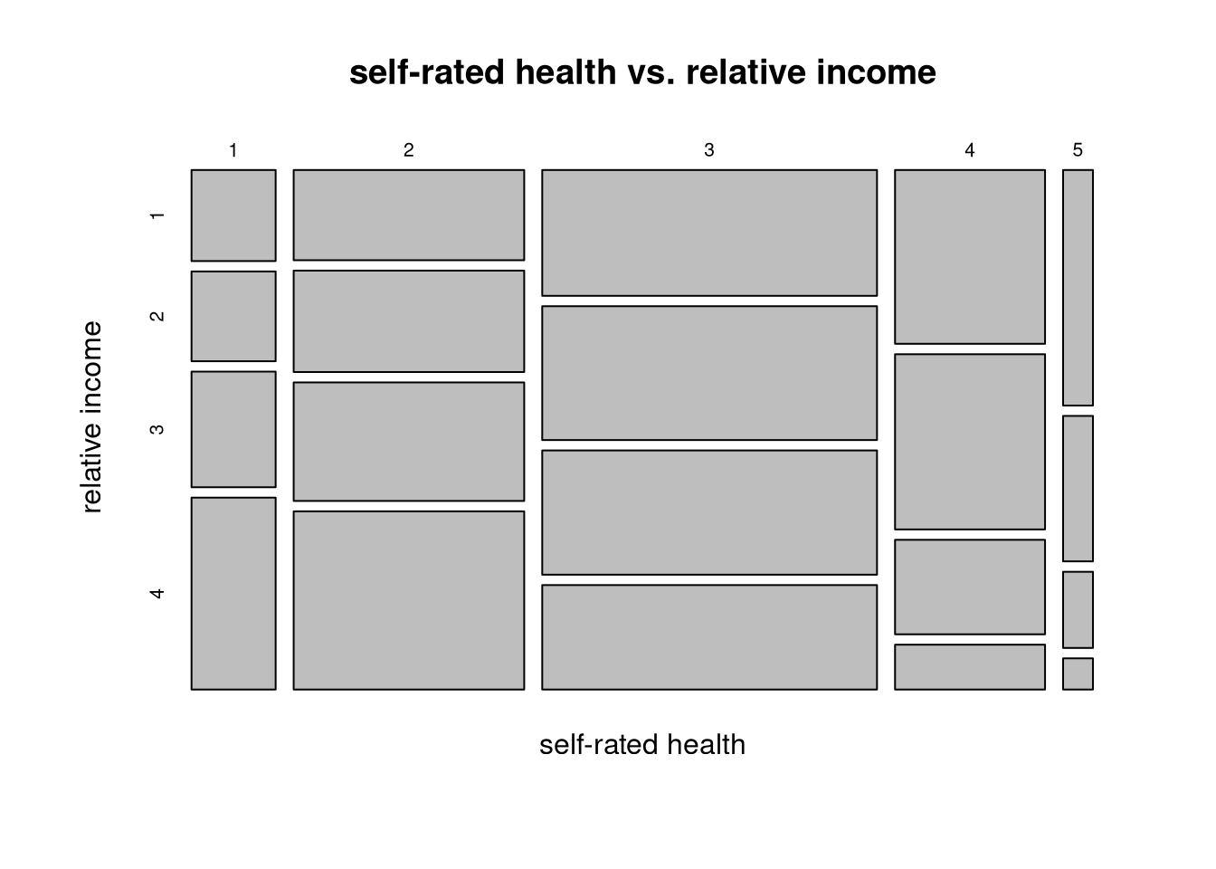
Task 4.6
Test the relation for statistical significance using an appropriate test.
chisq.test(dat$srhgnrl, dat$increl)
    Pearson's Chi-squared test

data:  dat$srhgnrl and dat$increl
X-squared = 335.89, df = 12, p-value < 2.2e-16
Task 4.7
Categorize the variable bmi into an underweight (BMI<18.5), normal weight (18.5≤BMI<25), overweight (25≤BMI<30) and obese (BMI≥30) group. Turn the variable into a factor.
line
Task 4.8
What is the proportion of overweight or obese people according to the categorized BMI? What is the proportion of people ever diagnosed with being overweight (variable ovrwght_ever)? How many overweight people were actually ever diagnosed with being overweight?
bmi_cat <- NULL
bmi_cat[dat$bmi<18.5] <- "Underweight"
bmi_cat[dat$bmi>=18.5&dat$bmi<25] <- "Normal weight"
bmi_cat[dat$bmi>=25&dat$bmi<30] <- "Overweight"
bmi_cat[dat$bmi>=30] <- "Obese"
bmi_cat <- as.factor(bmi_cat)
dat$bmi_cat <- bmi_cat
prop.table(table(dat$ovrwght_ever))
    FALSE      TRUE
0.6848109 0.3151891 prop.table(table(dat$ovrwght_ever, dat$bmi_cat), margin = 2)
        Normal weight     Obese Overweight Underweight
  FALSE     0.9671907 0.3321033  0.7632275   1.0000000
  TRUE      0.0328093 0.6678967  0.2367725   0.0000000
Task 4.9
Is there a difference in diabetes prevalence between obese people diagnosed with overweight and those who were never diagnosed? What about self-rated health? How do you explain the results?
(tab <- table(dat$diab_lft[dat$bmi_cat=="Obese"], dat$ovrwght_ever[bmi_cat=="Obese"]))
    FALSE TRUE
  1   473  694
  2     0    7
3 48 253fisher.test(tab)
    Fisher's Exact Test for Count Data

data:  tab
p-value < 2.2e-16
alternative hypothesis: two.sided
(tab <- table(dat$srhgnrl[bmi_cat=="Obese"], dat$ovrwght_ever[bmi_cat=="Obese"]))
    FALSE TRUE
  1    39   34
  2    98  188
  3   237  435
  4    98  283
5 9 65prop.table(tab, margin=1)
        FALSE      TRUE
  1 0.5342466 0.4657534
  2 0.3426573 0.6573427
  3 0.3526786 0.6473214
  4 0.2572178 0.7427822
  5 0.1216216 0.8783784
# Chi-square trend test
chisq.test(tab)
    Pearson's Chi-squared test

data:  tab
X-squared = 39.326, df = 4, p-value = 5.966e-08